Other random effects structures

Preliminaries

Open Rstudio, and create a new RMarkdown document (giving it a title for this week).

Non-convergence and singular fits: what should I do?

Singular fits

You may have noticed that a lot of our models over the last few weeks have been giving a warning: boundary (singular) fit: see ?isSingular.
Up to now, we’ve been largely ignoring these warnings. However, this week we’re going to look at how to deal with this issue.

The warning is telling us that our model has resulted in a ‘singular fit.’ Singular fits often indicate that the model is ‘overfitted’ - that is, the random effects structure which we have specified is too complex to be supported by the data.

Perhaps the most intuitive advice would be remove the most complex part of the random effects structure (i.e. random slopes). This leads to a simpler model that is not over-fitted. In other words, start simplying from the top (where the most complexity is) to the bottom (where the lowest complexity is). Additionally, when variance estimates are very low for a specific random effect term, this indicates that the model is not estimating this parameter to differ much between the levels of your grouping variable. It might, in some experimental designs, be perfectly acceptable to remove this or simply include it as a fixed effect.

A key point here is that when fitting a mixed model, we should think about how the data are generated. Asking yourself questions such as “do we have good reason to assume subjects might vary over time, or to assume that they will have different starting points (i.e., different intercepts)?” can help you in specifying your random effect structure

You can read in depth about what this means by reading the help documentation for ?isSingular. For our purposes, a relevant section is copied below:

… intercept-only models, or 2-dimensional random effects such as intercept + slope models, singularity is relatively easy to detect because it leads to random-effect variance estimates of (nearly) zero, or estimates of correlations that are (almost) exactly -1 or 1.

Convergence warnings

Issues of non-convergence can be caused by many things. If you’re model doesn’t converge, it does not necessarily mean the fit is incorrect, however it is is cause for concern, and should be addressed, else you may end up reporting inferences which do not hold.

There are lots of different things which you could do which might help your model to converge. A select few are detailed below:

• double-check the model specification and the data

• adjust stopping (convergence) tolerances for the nonlinear optimizer, using the optCtrl argument to [g]lmerControl. (see ?convergence for convergence controls).

  • What is “tolerance?” Remember that our optimizer is the the method by which the computer finds the best fitting model, by iteratively assessing and trying to maximise the likelihood (or minimise the loss).
    

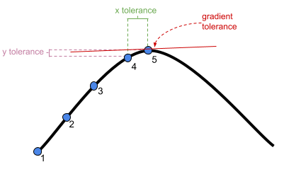
    Figure 1: An optimizer will stop after a certain number of iterations, or when it meets a tolerance threshold

• center and scale continuous predictor variables (e.g. with scale)

• Change the optimization method (for example, here we change it to bobyqa): lmer(..., control = lmerControl(optimizer="bobyqa"))
glmer(..., control = glmerControl(optimizer="bobyqa"))

• Increase the number of optimization steps: lmer(..., control = lmerControl(optimizer="bobyqa", optCtrl=list(maxfun=50000))
glmer(..., control = glmerControl(optimizer="bobyqa", optCtrl=list(maxfun=50000))

• Use allFit() to try the fit with all available optimizers. This will of course be slow, but is considered ‘the gold standard’; “if all optimizers converge to values that are practically equivalent, then we would consider the convergence warnings to be false positives.”

Random effects

When specifying a random effects model, think about the data you have and how they fit in the following table:

Criterion:	Repetition: If the experiment were repeated:	Desired inference: The conclusions refer to:
Fixed effects	Same levels would be used	The levels used
Random effects	Different levels would be used	A population from which the levels used are just a (random) sample

For example, applying the criteria to the following questions:

• Do dogs learn faster with higher rewards?

  FIXED: reward

  RANDOM: dog

• Do students read faster at higher temperatures?

  FIXED: temperature

  RANDOM: student

• Does people speaking one language speak faster than another?

  FIXED: the language

  RANDOM: the people speaking that language

Sometimes, after simplifying the model, you find that there isn’t much variability in a specific random effect and, if it still leads to singular fits or convergence warnings, it is common to just model that variable as a fixed effect.

Other times, you don’t have sufficient data or levels to estimate the random effect variance, and you are forced to model it as a fixed effect. This is similar to trying to find the “best-fit” line passing through a single point… You can’t because you need two points!

Random effects in lme4

Below are a selection of different formulas for specifying different random effect structures, taken from the lme4 vignette. This might look like a lot, but over time and repeated use of multilevel models you will get used to reading these in a similar way to getting used to reading the formula structure of y ~ x1 + x2 in all our linear models.

Formula	Alternative	Meaning
\(\text{(1 | g)}\)	\(\text{1 + (1 | g)}\)	Random intercept with fixed mean
\(\text{0 + offset(o) + (1 | g)}\)	\(\text{-1 + offset(o) + (1 | g)}\)	Random intercept with a priori means
\(\text{(1 | g1/g2)}\)	\(\text{(1 | g1) + (1 | g1:g2)}\)	Intercept varying among \(g1\) and \(g2\) within \(g1\)
\(\text{(1 | g1) + (1 | g2)}\)	\(\text{1 + (1 | g1) + (1 | g2)}\)	Intercept varying among \(g1\) and \(g2\)
\(\text{x + (x | g)}\)	\(\text{1 + x + (1 + x | g)}\)	Correlated random intercept and slope
\(\text{x + (x || g)}\)	\(\text{1 + x + (x | g) + (0 + x | g)}\)	Uncorrelated random intercept and slope

Table 1: Examples of the right-hand-sides of mixed effects model formulas. \(g\), \(g1\), \(g2\) are grouping factors, covariates and a priori known offsets are \(x\) and \(o\).

A. Three-level nesting

Data Codebook: Treatment effects

Synthetic data from a RCT treatment study: 5 therapists randomly assigned participants to control or treatment group and monitored the participants’ performance over time. There was a baseline test, then 6 weeks of treatment, with test sessions every week (7 total sessions).

The following code will load in your R session an object already called tx with the data:

load(url("https://uoepsy.github.io/msmr/data/tx.Rdata"))

You can see the head of the data below:

group	session	therapist	Score	PID
control	1	A	0.56	A_control_15
control	1	B	0.61	B_control_15
control	1	C	0.54	C_control_15
control	1	D	0.45	D_control_15
control	1	E	0.59	E_control_15
control	1	A	0.56	A_control_21

Question 1

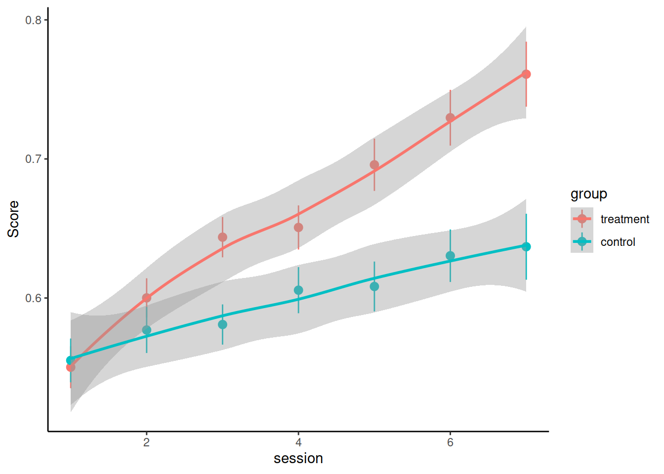
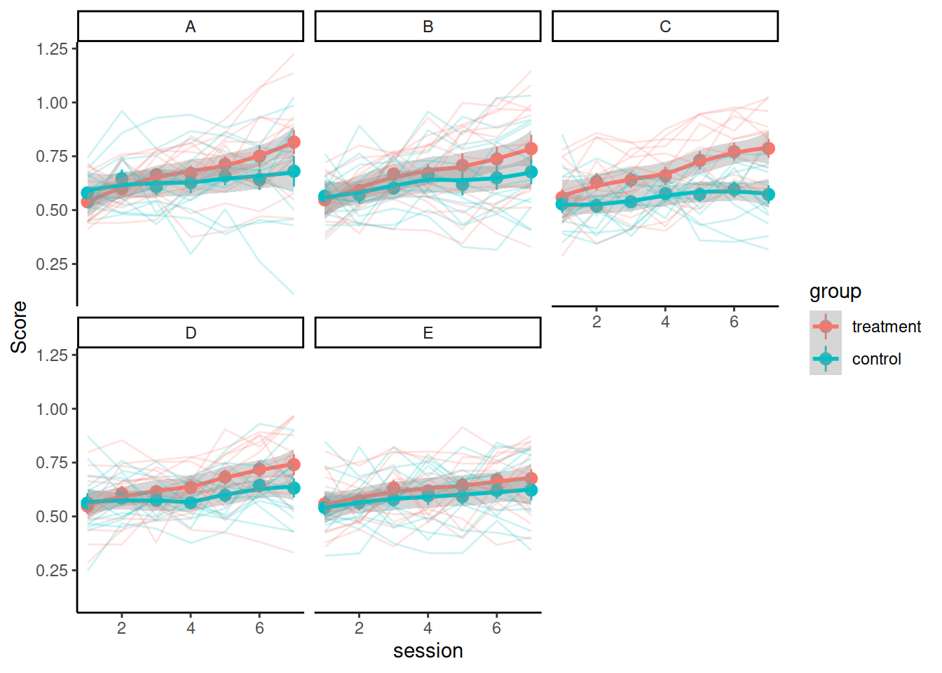
Load and visualise the data. Does it look like the treatment had an effect on the performance score?

Solution

ggplot(tx, aes(session, Score, color=group)) +
  stat_summary(fun.data = mean_se, geom="pointrange") +
  stat_smooth() +
  theme_classic()

Just for fun, let’s add on the individual participant scores, and also make a plot for each therapist.

ggplot(tx, aes(session, Score, color=group)) +
  stat_summary(fun.data = mean_se, geom = "pointrange") +
  stat_smooth() +
  theme_classic() +
  geom_line(aes(group = PID), alpha = .2) + 
  facet_wrap(~ therapist)

Question 2

Consider these questions when you’re designing your model(s) and use your answers to motivate your model design and interpretation of results:

1. What are the levels of nesting? How should that be reflected in the random effect structure?
2. What is the shape of change over time? Do you need polynomials to model this shape? If yes, what order polynomials?

Solution

1. There are repeated measures of participants (session). There are also repeated measures of therapists (each one treated many participants).
2. Looks like linear change, don’t need polynomials. Good to know that there is no difference at baseline, so no need for orthogonal time.

Question 3

Test whether the treatment had an effect using mixed-effects modelling.

Try to fit the maximal model.
Does it converge? Is it singular?

Hint: What is the maximal model?

There’s an interaction between session and group. Each participant has several sessions, so we want (1 + session | PID) and each therapist has several groups and sessions, so we want (1 + ? * ? | ?)

Solution

library(lme4)
library(lmerTest)

# start with maximal model
m1 <- lmer(Score ~ session * group + 
             (1 + session | PID) + 
             (1 + session * group | therapist),
           data=tx, REML=FALSE)

isSingular(m1)

## [1] TRUE

Question 4

Try adjusting your model by removing random effects or correlations, examine the model again, and so on..

Solution

VarCorr(m1)

##  Groups    Name                 Std.Dev.   Corr                
##  PID       (Intercept)          0.11715958                     
##            session              0.03137359 -0.601              
##  therapist (Intercept)          0.00000000                     
##            session              0.00069241    NaN              
##            groupcontrol         0.00290504    NaN  1.000       
##            session:groupcontrol 0.00058153    NaN -1.000 -1.000
##  Residual                       0.07326948

There’s a correlation of exactly -1 between the random intercepts and slopes for therapists, and the standard deviation estimate for session|therapist is pretty small. Let’s remove it.

m2 <- lmer(Score ~ session * group + 
             (1 + session | PID) + 
             (1 | therapist),
           data=tx, REML=FALSE)
VarCorr(m2)

##  Groups    Name        Std.Dev. Corr  
##  PID       (Intercept) 0.11717        
##            session     0.03138  -0.601
##  therapist (Intercept) 0.00000        
##  Residual              0.07327

It now looks like estimates for random intercepts for therapists is now 0. If we remove this, our model finally is non-singular:

m3 <- lmer(Score ~ session * group + 
             (1 + session | PID),
           data=tx, REML=FALSE)
summary(m3)

## Linear mixed model fit by maximum likelihood . t-tests use Satterthwaite's
##   method [lmerModLmerTest]
## Formula: Score ~ session * group + (1 + session | PID)
##    Data: tx
## 
##      AIC      BIC   logLik deviance df.resid 
##  -1649.8  -1611.0    832.9  -1665.8      937 
## 
## Scaled residuals: 
##      Min       1Q   Median       3Q      Max 
## -2.63288 -0.58802  0.01438  0.55505  2.87865 
## 
## Random effects:
##  Groups   Name        Variance  Std.Dev. Corr 
##  PID      (Intercept) 0.0137300 0.11717       
##           session     0.0009848 0.03138  -0.60
##  Residual             0.0053685 0.07327       
## Number of obs: 945, groups:  PID, 135
## 
## Fixed effects:
##                        Estimate Std. Error         df t value Pr(>|t|)    
## (Intercept)            0.526849   0.015841 135.002803  33.260  < 2e-16 ***
## session                0.033688   0.004100 134.995010   8.217 1.51e-13 ***
## groupcontrol           0.018136   0.022829 135.002805   0.794 0.428332    
## session:groupcontrol  -0.020138   0.005908 134.995014  -3.409 0.000861 ***
## ---
## Signif. codes:  0 '***' 0.001 '**' 0.01 '*' 0.05 '.' 0.1 ' ' 1
## 
## Correlation of Fixed Effects:
##             (Intr) sessin grpcnt
## session     -0.655              
## groupcontrl -0.694  0.454       
## sssn:grpcnt  0.454 -0.694 -0.655

Lastly, it’s then a good idea to check that the parameter estimates and SE are not radically different across these models (they are virtually identical)

summary(m1)$coefficients

##                         Estimate  Std. Error        df   t value     Pr(>|t|)
## (Intercept)           0.52684907 0.015838899 134.71030 33.262986 7.987774e-67
## session               0.03368821 0.004110515  49.18334  8.195617 9.353263e-11
## groupcontrol          0.01813605 0.022863224  95.49304  0.793241 4.296040e-01
## session:groupcontrol -0.02013829 0.005912772 111.37780 -3.405897 9.180515e-04

summary(m2)$coefficients

##                         Estimate  Std. Error       df    t value     Pr(>|t|)
## (Intercept)           0.52684907 0.015840448 135.0046 33.2597335 6.641086e-67
## session               0.03368821 0.004099564 135.0029  8.2175099 1.507171e-13
## groupcontrol          0.01813605 0.022828515 135.0046  0.7944471 4.283295e-01
## session:groupcontrol -0.02013829 0.005908101 135.0029 -3.4085898 8.611531e-04

summary(m3)$coefficients

##                         Estimate  Std. Error       df    t value     Pr(>|t|)
## (Intercept)           0.52684907 0.015840534 135.0028 33.2595529 6.653281e-67
## session               0.03368821 0.004099663 134.9950  8.2173108 1.509284e-13
## groupcontrol          0.01813605 0.022828639 135.0028  0.7944428 4.283320e-01
## session:groupcontrol -0.02013829 0.005908244 134.9950 -3.4085072 8.614061e-04

Extra: Question 5

Try the code below to use the allFit() function to fit your final model with all the available optimizers.¹

• You might need to install the dfoptim package to get one of the optimizers

sumfits <- allFit(yourmodel)
summary(sumfits)

B. Crossed random effects

Data Codeook: Test-enhanced learning

An experiment was run to replicate “test-enhanced learning” (Roediger & Karpicke, 2006): two groups of 25 participants were presented with material to learn. One group studied the material twice (StudyStudy), the other group studied the material once then did a test (StudyTest). Recall was tested immediately (one minute) after the learning session and one week later. The recall tests were composed of 175 items identified by a keyword (Test_word).

The critical (replication) prediction is that the StudyStudy group should perform somewhat better on the immediate recall test, but the StudyTest group will retain the material better and thus perform better on the 1-week follow-up test.

The following code loads the data into your R environment by creating a variable called tel:

load(url("https://uoepsy.github.io/msmr/data/TestEnhancedLearning.RData"))

The head of the dataset can be seen below:

Subject_ID	Group	Delay	Test_word	Correct
StudyTest_L	StudyTest	min	van	1
StudyTest_L	StudyTest	week	dinosaur	0
StudyTest_L	StudyTest	min	typewriter	0
StudyTest_L	StudyTest	min	chimney	0
StudyTest_L	StudyTest	week	dog	1
StudyTest_L	StudyTest	min	turkey	1

Question 6

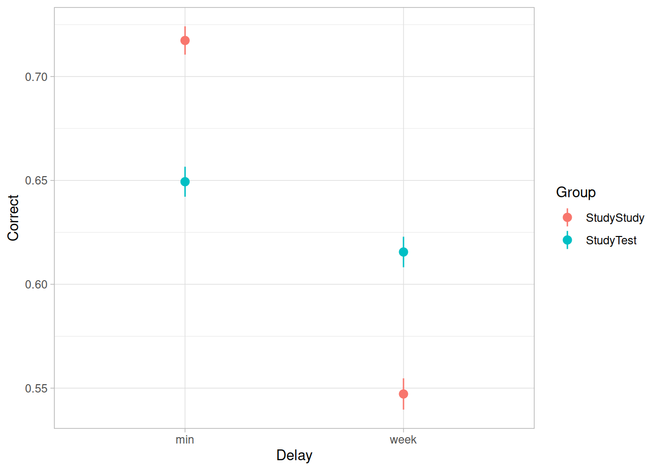
Load and plot the data. Does it look like the effect was replicated?

Solution

You can make use of stat_summary() again!

ggplot(tel, aes(Delay, Correct, col=Group)) + 
  stat_summary(fun.data=mean_se, geom="pointrange")+
  theme_light()

It’s more work, but some people might rather calculate the numbers and then plot them directly. It does just the same thing:

tel %>% 
  group_by(Delay, Group) %>%
  summarise(
    mean = mean(Correct),
    se = sd(Correct)/sqrt(n())
  ) %>%
  ggplot(., aes(x=Delay, col = Group)) +
  geom_pointrange(aes(y=mean, ymin=mean-se, ymax=mean+se))+
  theme_light() +
  labs(y = "Correct")

That looks like test-enhanced learning to me!

Question 7

Test the critical hypothesis using a mixed-effects model. Fit the maximal random effect structure supported by the experimental design.

Some questions to consider:

• Item accuracy is a binary variable. What kind of model will you use?
  

• We can expect variability across subjects (some people are better at learning than others) and across items (some of the recall items are harder than others). How should this be represented in the random effects?

• If a model takes ages to fit, you might want to cancel it by pressing the escape key. It is normal for complex models to take time, but for the purposes of this task, give up after a couple of minutes, and try simplifying your model.

Solution

This one will probably take too long:

m <- glmer(Correct ~ Delay*Group +
             (1 + Delay | Subject_ID) +
             (1 + Delay * Group | Test_word),
           data=tel, family="binomial",
           glmerControl(optimizer = "bobyqa"))

So lets remove the interaction in the by-word random effects:

m <- glmer(Correct ~ Delay*Group +
             (1 + Delay | Subject_ID) +
             (1 + Delay + Group | Test_word),
           data=tel, family="binomial",
           glmerControl(optimizer = "bobyqa"))
summary(m)

## Generalized linear mixed model fit by maximum likelihood (Laplace
##   Approximation) [glmerMod]
##  Family: binomial  ( logit )
## Formula: Correct ~ Delay * Group + (1 + Delay | Subject_ID) + (1 + Delay +  
##     Group | Test_word)
##    Data: tel
## Control: glmerControl(optimizer = "bobyqa")
## 
##      AIC      BIC   logLik deviance df.resid 
##  16289.8  16390.8  -8131.9  16263.8    17485 
## 
## Scaled residuals: 
##     Min      1Q  Median      3Q     Max 
## -7.4352 -0.4778  0.2763  0.5182  7.5360 
## 
## Random effects:
##  Groups     Name           Variance Std.Dev. Corr       
##  Test_word  (Intercept)    1.160006 1.07704             
##             Delayweek      0.005544 0.07446  -0.80      
##             GroupStudyTest 0.011906 0.10911  -0.93  0.97
##  Subject_ID (Intercept)    2.527060 1.58967             
##             Delayweek      0.044398 0.21071  -0.60      
## Number of obs: 17498, groups:  Test_word, 175; Subject_ID, 50
## 
## Fixed effects:
##                          Estimate Std. Error z value Pr(>|z|)    
## (Intercept)               1.28218    0.33086   3.875 0.000107 ***
## Delayweek                -1.07133    0.07068 -15.157  < 2e-16 ***
## GroupStudyTest           -0.42871    0.45380  -0.945 0.344804    
## Delayweek:GroupStudyTest  0.79434    0.10191   7.795 6.47e-15 ***
## ---
## Signif. codes:  0 '***' 0.001 '**' 0.01 '*' 0.05 '.' 0.1 ' ' 1
## 
## Correlation of Fixed Effects:
##             (Intr) Delywk GrpStT
## Delayweek   -0.441              
## GropStdyTst -0.688  0.309       
## Dlywk:GrpST  0.292 -0.679 -0.430
## optimizer (bobyqa) convergence code: 0 (OK)
## boundary (singular) fit: see ?isSingular

Question 8

The model with maximal random effects will probably not converge, or will obtain a singular fit. Simplify the model until you achieve convergence.

What we’re aiming to do here is to follow Barr et al.’s advice of defining our maximal model and then removing only the terms to allow a non-singular fit.

Note: This strategy - starting with the maximal random effects structure and removing terms until obtaining model convergence, is just one approach, and there are drawbacks (see Matuschek et al., 2017). There is no consensus on what approach is best (see ?isSingular).


Tip: you can look at the variance estimates and correlations easily by using the VarCorr() function. What jumps out?

Hint: Generalization over subjects could be considered more important than over items - if the estimated variance of slopes for Delay and Group by-items are comparatively small, it might be easier to remove them?

Solution

VarCorr(m)

##  Groups     Name           Std.Dev. Corr         
##  Test_word  (Intercept)    1.077036              
##             Delayweek      0.074456 -0.803       
##             GroupStudyTest 0.109113 -0.930  0.966
##  Subject_ID (Intercept)    1.589673              
##             Delayweek      0.210709 -0.600

The by-item slope of Group seems to be quite highly correlated with other by-item terms.

For now, we will just simply remove the term (however, we could - if we had theoretical justification - constrain our model so that there was 0 correlation)

m2 <- glmer(Correct ~ Delay*Group +
             (1 + Delay | Subject_ID) +
             (1 + Delay | Test_word),
            data=tel, family="binomial",
            glmerControl(optimizer = "bobyqa"))
VarCorr(m2)

##  Groups     Name        Std.Dev. Corr  
##  Test_word  (Intercept) 1.027504       
##             Delayweek   0.055414 -1.000
##  Subject_ID (Intercept) 1.598992       
##             Delayweek   0.208731 -0.599

It’s still a singular fit, and the Delay random slope by Test_word variance is extremely low and perfectly correlated with the intercept, let’s try removing that:

m3 <- glmer(Correct ~ Delay*Group +
              (1 + Delay | Subject_ID) +
              (1 | Test_word),
            data=tel, family="binomial",
            glmerControl(optimizer = "bobyqa"))

Hooray, the model converged!

summary(m3)

## Generalized linear mixed model fit by maximum likelihood (Laplace
##   Approximation) [glmerMod]
##  Family: binomial  ( logit )
## Formula: Correct ~ Delay * Group + (1 + Delay | Subject_ID) + (1 | Test_word)
##    Data: tel
## Control: glmerControl(optimizer = "bobyqa")
## 
##      AIC      BIC   logLik deviance df.resid 
##  16285.3  16347.4  -8134.6  16269.3    17490 
## 
## Scaled residuals: 
##     Min      1Q  Median      3Q     Max 
## -7.5190 -0.4795  0.2758  0.5199  8.0698 
## 
## Random effects:
##  Groups     Name        Variance Std.Dev. Corr 
##  Test_word  (Intercept) 0.9961   0.9980        
##  Subject_ID (Intercept) 2.5170   1.5865        
##             Delayweek   0.0387   0.1967   -0.52
## Number of obs: 17498, groups:  Test_word, 175; Subject_ID, 50
## 
## Fixed effects:
##                          Estimate Std. Error z value Pr(>|z|)    
## (Intercept)               1.25717    0.32858   3.826  0.00013 ***
## Delayweek                -1.04684    0.06750 -15.508  < 2e-16 ***
## GroupStudyTest           -0.39818    0.45252  -0.880  0.37890    
## Delayweek:GroupStudyTest  0.77633    0.09916   7.829 4.92e-15 ***
## ---
## Signif. codes:  0 '***' 0.001 '**' 0.01 '*' 0.05 '.' 0.1 ' ' 1
## 
## Correlation of Fixed Effects:
##             (Intr) Delywk GrpStT
## Delayweek   -0.371              
## GropStdyTst -0.687  0.267       
## Dlywk:GrpST  0.252 -0.679 -0.371

Question 9

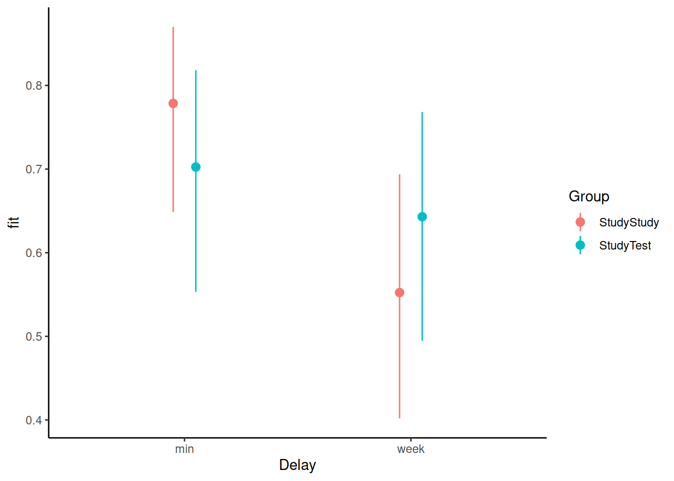
Load the effects package, and try running this code:

library(effects)
ef <- as.data.frame(effect("Delay:Group", m3))

What is ef? and how can you use it to plot the model-estimated condition means and variability?

Solution

ggplot(ef, aes(Delay, fit, color=Group)) + 
  geom_pointrange(aes(ymax=upper, ymin=lower), position=position_dodge(width = 0.2))+
  theme_classic() # just for a change :)

Question 10

What should we do with this information? How can we apply test-enhanced learning to learning R and statistics?

Solution

You’ll get the benefits of test-enhanced learning if you try yourself before looking at the solutions! If you don’t test yourself, you’re more likely to forget it in the long run.

Suggested readings (optional)

• Baayen et al., 2008
  
• Barr et al., 2013
  
• Matuschek et al., 2017

---

1. If you have an older version of lme4, then allFit() might not be directly available, and you will need to run the following: source(system.file("utils", "allFit.R", package="lme4")).↩︎