optional eigen decomp

Doing data reduction can feel a bit like magic, and in part that’s just because it’s quite complicated.

The intuition

Consider one way we might construct a correlation matrix - as the product of vector \(\mathbf{f}\) with \(\mathbf{f'}\) (f transposed): \[ \begin{equation*} \mathbf{f} = \begin{bmatrix} 0.9 \\ 0.8 \\ 0.7 \\ 0.6 \\ 0.5 \\ 0.4 \\ \end{bmatrix} \qquad \mathbf{f} \mathbf{f'} = \begin{bmatrix} 0.9 \\ 0.8 \\ 0.7 \\ 0.6 \\ 0.5 \\ 0.4 \\ \end{bmatrix} \begin{bmatrix} 0.9, 0.8, 0.7, 0.6, 0.5, 0.4 \\ \end{bmatrix} \qquad = \qquad \begin{bmatrix} 0.81, 0.72, 0.63, 0.54, 0.45, 0.36 \\ 0.72, 0.64, 0.56, 0.48, 0.40, 0.32 \\ 0.63, 0.56, 0.49, 0.42, 0.35, 0.28 \\ 0.54, 0.48, 0.42, 0.36, 0.30, 0.24 \\ 0.45, 0.40, 0.35, 0.30, 0.25, 0.20 \\ 0.36, 0.32, 0.28, 0.24, 0.20, 0.16 \\ \end{bmatrix} \end{equation*} \]

But we constrain this such that the diagonal has values of 1 (the correlation of a variable with itself is 1), and lets call it R. \[ \begin{equation*} \mathbf{R} = \begin{bmatrix} 1.00, 0.72, 0.63, 0.54, 0.45, 0.36 \\ 0.72, 1.00, 0.56, 0.48, 0.40, 0.32 \\ 0.63, 0.56, 1.00, 0.42, 0.35, 0.28 \\ 0.54, 0.48, 0.42, 1.00, 0.30, 0.24 \\ 0.45, 0.40, 0.35, 0.30, 1.00, 0.20 \\ 0.36, 0.32, 0.28, 0.24, 0.20, 1.00 \\ \end{bmatrix} \end{equation*} \]

PCA is about trying to determine a vector f which generates the correlation matrix R. a bit like unscrambling eggs!

in PCA, we express \(\mathbf{R = CC'}\), where \(\mathbf{C}\) are our principal components.
If \(n\) is number of variables in \(R\), then \(i^{th}\) component \(C_i\) is the linear sum of each variable multiplied by some weighting:
\[ C_i = \sum_{j=1}^{n}w_{ij}x_{j} \]

How do we find \(C\)?

This is where “eigen decomposition” comes in.
For the \(n \times n\) correlation matrix \(\mathbf{R}\), there is an eigenvector \(x_i\) that solves the equation \[ \mathbf{x_i R} = \lambda_i \mathbf{x_i} \] Where the vector multiplied by the correlation matrix is equal to some eigenvalue \(\lambda_i\) multiplied by that vector.
We can write this without subscript \(i\) as: \[ \begin{align} & \mathbf{R X} = \mathbf{X \lambda} \\ & \text{where:} \\ & \mathbf{R} = \text{correlation matrix} \\ & \mathbf{X} = \text{matrix of eigenvectors} \\ & \mathbf{\lambda} = \text{vector of eigenvalues} \end{align} 
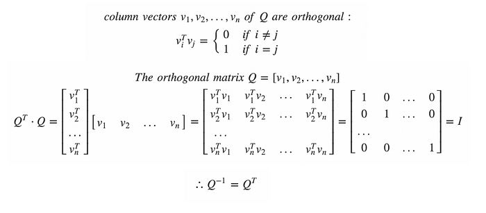
\] the vectors which make up \(\mathbf{X}\) must be orthogonal (\(\mathbf{XX' = I}\)), which means that \(\mathbf{R = X \lambda X'}\)

We can actually do this in R manually. Creating a correlation matrix

# lets create a correlation matrix, as the produce of ff'
f <- seq(.9,.4,-.1)
R <- f %*% t(f)
#give rownames and colnames
rownames(R)<-colnames(R)<-paste0("V",seq(1:6))
#constrain diagonals to equal 1
diag(R)<-1
R
     V1   V2   V3   V4   V5   V6
V1 1.00 0.72 0.63 0.54 0.45 0.36
V2 0.72 1.00 0.56 0.48 0.40 0.32
V3 0.63 0.56 1.00 0.42 0.35 0.28
V4 0.54 0.48 0.42 1.00 0.30 0.24
V5 0.45 0.40 0.35 0.30 1.00 0.20
V6 0.36 0.32 0.28 0.24 0.20 1.00

Eigen Decomposition

# do eigen decomposition
e <- eigen(R)
print(e, digits=2)
eigen() decomposition
$values
[1] 3.16 0.82 0.72 0.59 0.44 0.26

$vectors
      [,1]   [,2]   [,3]  [,4]   [,5]   [,6]
[1,] -0.50 -0.061  0.092  0.14  0.238  0.816
[2,] -0.47 -0.074  0.121  0.21  0.657 -0.533
[3,] -0.43 -0.096  0.182  0.53 -0.675 -0.184
[4,] -0.39 -0.142  0.414 -0.78 -0.201 -0.104
[5,] -0.34 -0.299 -0.860 -0.20 -0.108 -0.067
[6,] -0.28  0.934 -0.178 -0.10 -0.067 -0.045

The eigenvectors are orthogonal (\(\mathbf{XX' = I}\)):

round(e$vectors %*% t(e$vectors),2)
     [,1] [,2] [,3] [,4] [,5] [,6]
[1,]    1    0    0    0    0    0
[2,]    0    1    0    0    0    0
[3,]    0    0    1    0    0    0
[4,]    0    0    0    1    0    0
[5,]    0    0    0    0    1    0
[6,]    0    0    0    0    0    1

The Principal Components \(\mathbf{C}\) are the eigenvectors scaled by the square root of the eigenvalues:

#eigenvectors
e$vectors
       [,1]    [,2]    [,3]   [,4]    [,5]    [,6]
[1,] -0.496 -0.0611  0.0923  0.139  0.2385  0.8155
[2,] -0.468 -0.0743  0.1210  0.214  0.6566 -0.5327
[3,] -0.433 -0.0963  0.1820  0.530 -0.6751 -0.1842
[4,] -0.390 -0.1416  0.4143 -0.778 -0.2006 -0.1036
[5,] -0.340 -0.2992 -0.8604 -0.197 -0.1076 -0.0669
[6,] -0.282  0.9338 -0.1784 -0.100 -0.0667 -0.0452
#scaled by sqrt of eigenvalues
diag(sqrt(e$values))
     [,1]  [,2]  [,3]  [,4]  [,5]  [,6]
[1,] 1.78 0.000 0.000 0.000 0.000 0.000
[2,] 0.00 0.906 0.000 0.000 0.000 0.000
[3,] 0.00 0.000 0.848 0.000 0.000 0.000
[4,] 0.00 0.000 0.000 0.769 0.000 0.000
[5,] 0.00 0.000 0.000 0.000 0.664 0.000
[6,] 0.00 0.000 0.000 0.000 0.000 0.512
C <- e$vectors %*% diag(sqrt(e$values))
C
       [,1]    [,2]    [,3]    [,4]    [,5]    [,6]
[1,] -0.883 -0.0554  0.0782  0.1070  0.1584  0.4174
[2,] -0.833 -0.0673  0.1025  0.1648  0.4361 -0.2727
[3,] -0.770 -0.0873  0.1542  0.4077 -0.4483 -0.0943
[4,] -0.694 -0.1284  0.3512 -0.5987 -0.1332 -0.0530
[5,] -0.604 -0.2712 -0.7293 -0.1514 -0.0715 -0.0342
[6,] -0.502  0.8464 -0.1513 -0.0771 -0.0443 -0.0231

And we can reproduce our correlation matrix, because \(\mathbf{R = CC'}\).

C %*% t(C)
     [,1] [,2] [,3] [,4] [,5] [,6]
[1,] 1.00 0.72 0.63 0.54 0.45 0.36
[2,] 0.72 1.00 0.56 0.48 0.40 0.32
[3,] 0.63 0.56 1.00 0.42 0.35 0.28
[4,] 0.54 0.48 0.42 1.00 0.30 0.24
[5,] 0.45 0.40 0.35 0.30 1.00 0.20
[6,] 0.36 0.32 0.28 0.24 0.20 1.00

Now lets imagine we only consider 1 principal component.
We can do this with the principal() function:

library(psych)
pc1<-principal(R, nfactors = 1, covar = FALSE, rotate = 'none')
pc1
Principal Components Analysis
Call: principal(r = R, nfactors = 1, rotate = "none", covar = FALSE)
Standardized loadings (pattern matrix) based upon correlation matrix
    PC1   h2   u2 com
V1 0.88 0.78 0.22   1
V2 0.83 0.69 0.31   1
V3 0.77 0.59 0.41   1
V4 0.69 0.48 0.52   1
V5 0.60 0.37 0.63   1
V6 0.50 0.25 0.75   1

                PC1
SS loadings    3.16
Proportion Var 0.53

Mean item complexity =  1
Test of the hypothesis that 1 component is sufficient.

The root mean square of the residuals (RMSR) is  0.09 

Fit based upon off diagonal values = 0.95

Look familiar? It looks like the first component we computed manually. The first column of \(\mathbf{C}\):

cbind(pc1$loadings, C=C[,1])
     PC1      C
V1 0.883 -0.883
V2 0.833 -0.833
V3 0.770 -0.770
V4 0.694 -0.694
V5 0.604 -0.604
V6 0.502 -0.502

We can now ask “how well does this component (on its own) recreate our correlation matrix?”

C[,1] %*% t(C[,1])
      [,1]  [,2]  [,3]  [,4]  [,5]  [,6]
[1,] 0.780 0.735 0.680 0.613 0.534 0.444
[2,] 0.735 0.693 0.641 0.578 0.503 0.418
[3,] 0.680 0.641 0.592 0.534 0.465 0.387
[4,] 0.613 0.578 0.534 0.481 0.419 0.348
[5,] 0.534 0.503 0.465 0.419 0.365 0.304
[6,] 0.444 0.418 0.387 0.348 0.304 0.252

It looks close, but not quite. How much not quite? Measurably so!

R - (C[,1] %*% t(C[,1]))
        V1      V2      V3      V4      V5      V6
V1  0.2200 -0.0154 -0.0498 -0.0727 -0.0838 -0.0836
V2 -0.0154  0.3067 -0.0809 -0.0976 -0.1033 -0.0982
V3 -0.0498 -0.0809  0.4075 -0.1140 -0.1153 -0.1066
V4 -0.0727 -0.0976 -0.1140  0.5187 -0.1193 -0.1085
V5 -0.0838 -0.1033 -0.1153 -0.1193  0.6346 -0.1036
V6 -0.0836 -0.0982 -0.1066 -0.1085 -0.1036  0.7477

Notice the values on the diagonals of \(\mathbf{c_1}\mathbf{c_1}'\).

diag(C[,1] %*% t(C[,1]))
[1] 0.780 0.693 0.592 0.481 0.365 0.252

These aren’t 1, like they are in \(R\). But they are proportional: this is the amount of variance in each observed variable that is explained by this first component. Sound familiar?

pc1$communality
   V1    V2    V3    V4    V5    V6 
0.780 0.693 0.592 0.481 0.365 0.252 

And likewise the 1 minus these is the unexplained variance:

1 - diag(C[,1] %*% t(C[,1]))
[1] 0.220 0.307 0.408 0.519 0.635 0.748
pc1$uniquenesses
   V1    V2    V3    V4    V5    V6 
0.220 0.307 0.408 0.519 0.635 0.748