W8: Sampling Distributions & Standard Error
Pick someone new to be the driver this week. If everyone in the group has already had a week as the driver, start going round again!
The driver will type the code. The rest of you are navigators, you need to tell the driver where to go (i.e., what to type!).
Driver instructions:
- Log in to the bigger screen at your table
- Open RStudio Server. See the first drop-down in the FAQs page for instructions
- Open a new .R script, and load the tidyverse package.
- Listen to your navigators
Navigator instructions:
- Tell your driver where to go (i.e., what to type)!
Question 1
This week’s workshop is a little bit more conceptual in nature. The steps that you work through here are not steps that you would use in an actual data analysis scenario. Instead, the goal is to help you get more comfortable thinking about the precision of a summary statistic like the mean.
Concretely, you’ll create your own sampling distributions based on a population we’ve simulated. And you’ll see that the standard deviation of those sampling distributions comes pretty close to giving the same result as the standard error formula you saw in the lecture! This tells us that the standard error is a reasonable way to calculate the precision of an estimate.
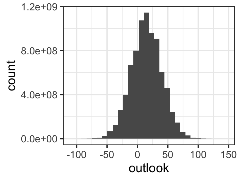
If our silly questionnaire was filled in by every person in the world, we would have billions of outlook scores that tell us how pessimistic vs. optimistic everybody in the world is on a scale from –100 to 100. That would be our population distribution. In real life, this is of course impossible, but for the exercises this week, we are going to imagine that we know the mean and standard deviation of the population distribution for outlook: the mean is 15 and the SD is 25.
Here’s what this imaginary population distribution looks like. (The numbers along the y axis use scientific notation: for example, 8e+08 means “eight followed by eight zeros”, or 800,000,000. These counts are huge because there are over eight billion people in the world!)
Now we are going draw samples from this population. We can generate a pretend sample of outlook scores by using the function rnorm().
Copy this code into your R script and (re)run it a few times. Is your fake sample and its mean different from ours? Is your fake sample different every time you run the code?
fake_sample <- rnorm(
  n = 5,        # how many data points do we want to sample?
  mean = 15,    # what's the mean of the distribution we're sampling from?
  sd = 25       # what's the SD of the distribution we're sampling from?
)
fake_sample
[1] -25.6906 73.0784 13.0881 -5.9601 2.7541mean(fake_sample)[1] 11.454
Question 2
You have hopefully noticed that every time we take a new pretend sample, the actual numbers it contains are different, and so is its mean. This point is key: the mean of each sample is a little bit different. This raises our next question: how different are those means?
To find out, we are going to take a LOT of samples from the population, find the mean of each one, and look at how spread-out they are. We’ll use the function replicate(), which lets us do something in R lots of times. Specifically, we’re going to draw and summarise 1000 samples.
Copy and run the following code.
means20 <- replicate(1000, mean(rnorm(n = 20, mean = 15, sd = 25)))

means100 <- replicate(1000, mean(rnorm(n = 100, mean = 15, sd = 25)))
Now, do your best to answer the following questions about this code (and ask a tutor if you’re not sure!):
- What part(s) of this code draws a random sample from the population distribution?
- Do all samples contain the same number of data points?
- What part(s) of this code calculates the mean of the sample?
- What part(s) of this code draws and summarises a sample 1000 times?
- Which of these two objects,
means20ormeans100, has more variability among the means it contains?
Question 3
In this question, you will prepare the two sampling distributions means20 and means100 for plotting.
Currently, means20 and means100 are both vectors. But ggplot doesn’t like vectors. It only likes dataframes, and so we are going to make two dataframes: one for means20 and another for means100. To make a dataframe, we’ll use the function tibble().
In the following code, replace the ... with the name of the appropriate vector. Then run the code.
data20 <- tibble(
  estimate = ...
)

data100 <- tibble(
  estimate = ...
)
The result should be two dataframes that each contain one column called estimate. In that column are the values that make up each of our sampling distributions.
🗂️ See Create a dataframe flash card.
Question 4
First, use ggplot to make two plots, one for each of these sampling distributions. What sort of plot? That’s up to you!
🗂️ See Plot a variable flash card.
Once you’ve made both lots, let’s display them side by side in the same graphic. To do this, we’ll need the patchwork package (and you might need to install it first!).
🗂️ See Use R packages flash card.
To arrange the plots side by side, you’ll need to:
- assign each plot a name, e.g.
plot1 <- ...andplot2 <- ..., and then - use
+to place them side by side (plot1 + plot2) or/to place one on top of the other (plot1 / plot2)
🗂️ See Patchwork flash card.
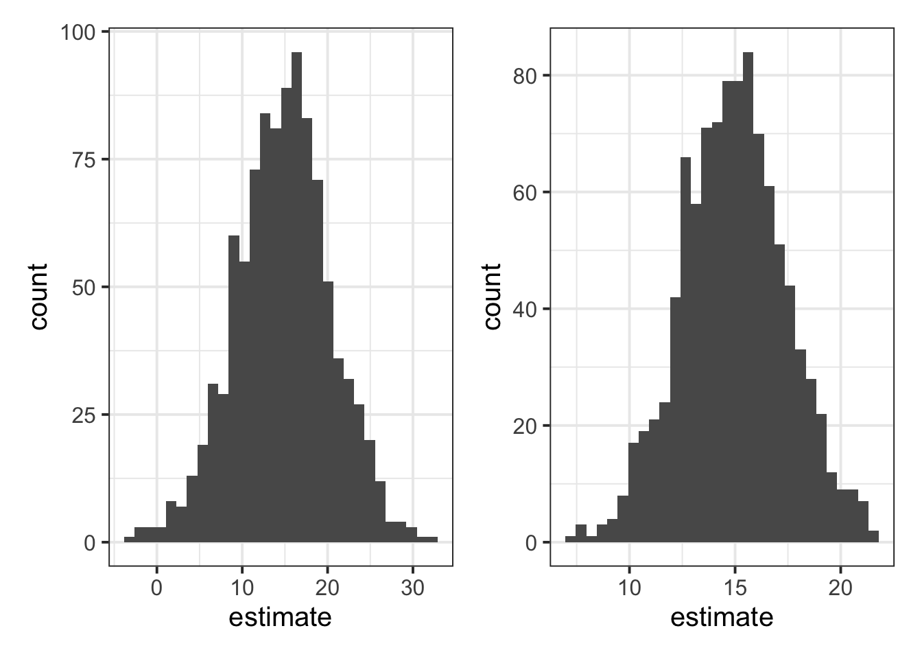
Each of the plots shows “means from 1000 samples we might see”, which is to say, they each show a sampling distribution of the mean. Rememebr that, because each sample is a random selection of people’s outlook scores, the means of the samples were different (some samples were full of more optimistic people, some with less optimistic people).
Now, do your best to answer the following questions (and ask a tutor if you’re not sure!):
- What differences do you see between the numbers in the plots you’ve made?
- Bonus challenge: Why are the numbers different?
Question 5
The goal of this final question is to show you that the standard deviation of the sampling distributions of the mean is pretty darn close to the standard error of the mean that we calculate using the following formula:
\[ SE_{\text{mean}} = \frac{\sigma}{\sqrt{n}} \]
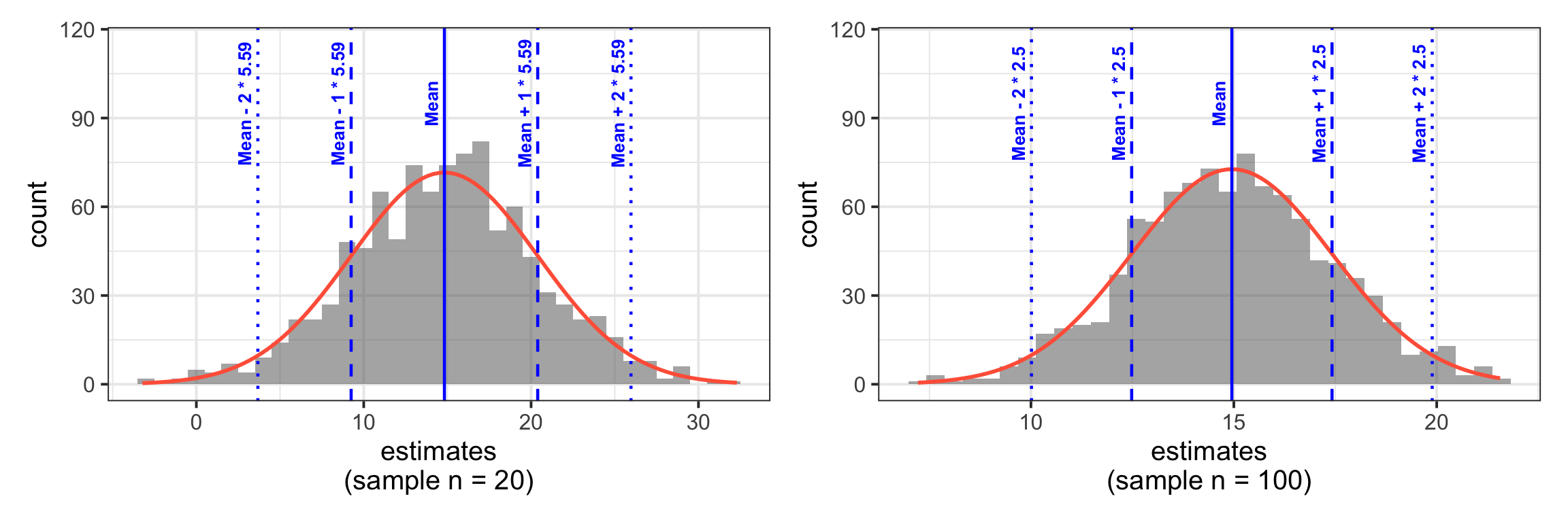
You saw in the lecture that the point of the standard error is to characterise “how much a sample estimate will vary due to random sampling”. And that’s exactly what our sampling distributions show as well! So it makes sense that they give us similar numbers.
Let’s see it in action. Here’s how we’d calculate the standard error of the mean, using our sample sizes of 20 and 100, our population mean of 15, and our population SD of 25:
\[ \begin{align} SE_{\text{mean, n=20}} &= \frac{25}{\sqrt{20}} \\ \quad \\ &= 5.59 \\ \end{align} \]
\[ \begin{align} SE_{\text{mean, n=100}} &= \frac{25}{\sqrt{100}} \\ \quad \\ &= 2.5 \\ \end{align} \]
Now, compute the standard deviation of the means from samples of size 20, as well as for the means from samples of size 100.
They won’t match exactly, but they should be close. And that’s why the standard error formula is so cool and useful! It lets us directly calculate how much sample means are going to vary, without needing to go through this long effortful sampling process.
🗂️ See Measure Variability > Standard deviation flash card.
Finishing up
Once you’ve finished, don’t forget to:
- Save your R script
- Post the R script to the group discussion space on Learn, to ensure that everyone has access to it! (For step-by-step instructions on how to do this, click here)