W5: Summarising Distributions II – Variability

Pick someone new to be the driver this week. They will type the code. The rest of you are navigators, you need to tell the driver where to go (i.e., what to type!).

Driver instructions:

1. Log in to the bigger screen at your table
2. Open RStudio Server. See the first drop-down in the FAQs page for instructions
3. Open a new .R script, and load the tidyverse package.
4. Listen to your navigators

Navigator instructions:

1. Tell your driver where to go (i.e., what to type)!

Question 1

We’re continuing to use the same dataset for the next couple of weeks (the survey that many of you completed in the first week). The data are stored at https://uoepsy.github.io/data/dapr1_2627_survey.csv (Check back to your work from the previous weeks to remind yourself how to get the data into R).

Calculate the Inter Quartile Range (IQR) for:

1. distance_born - the distances from Edinburgh that the respondents were born. The IQR is appropriate here because the variable is highly skewed.
   
2. spicy_num - the levels of spice that respondents like. The IQR is appropriate here because the variable is ordinal.

🗂️ See Measure variability > IQR flash card.

Solution 1.

library(tidyverse)
sdata <- read_csv("https://uoepsy.github.io/data/dapr1_2627_survey.csv")

sdata |> 
  summarise(
    dist_IQR = IQR(distance_born, na.rm = TRUE),
    spice_IQR = IQR(spicy_num, na.rm = TRUE)
  )

# A tibble: 1 × 2
  dist_IQR spice_IQR
     <dbl>     <dbl>
1     6659         1

Question 2

The survey also asked people to rate, on scales of 0 to 100, three things:

variable	question
sleepqual	“how well do you tend to sleep on average?”
procrast	“how often do you tend to procrastinate on tasks or responsibilities on average?”
multitask	“how well do you think you can handle multiple tasks or responsibilities at the same time on average?”

Calculate the mean and standard deviation for one of these variables.

🗂️ See Measure variability > SD flash card.

Solution 2.

sdata |> 
  summarise(
    sleep_M = mean(sleepqual, na.rm = TRUE),
    sleep_SD = sd(sleepqual, na.rm = TRUE),
    procr_M = mean(procrast, na.rm = TRUE),
    procr_SD = sd(procrast, na.rm = TRUE),
    mutli_M = mean(multitask, na.rm = TRUE),
    multi_SD = sd(multitask, na.rm = TRUE)
  )

# A tibble: 1 × 6
  sleep_M sleep_SD procr_M procr_SD mutli_M multi_SD
    <dbl>    <dbl>   <dbl>    <dbl>   <dbl>    <dbl>
1    55.4     20.3    60.6     25.5    56.5     21.2

Question 3

For the sleep-quality, procrastination, and multitasking variables, respondents were given the scale from 0 to 100. That doesn’t necessarily mean that people used the whole scale.

For the same variable you chose in the previous question, calculate its range.

🗂️ See Measure variability > Range flash card.

Solution 3. We’ve provided below the range of all 3 variables, so you can check your answer whichever one you chose.

sdata |> 
  summarise(
    sleep_R = max(sleepqual, na.rm = TRUE) - min(sleepqual, na.rm = TRUE),
    procr_R = max(procrast, na.rm = TRUE) - min(procrast, na.rm = TRUE),
    multi_R = max(multitask, na.rm = TRUE) - min(multitask, na.rm = TRUE)
  )

# A tibble: 1 × 3
  sleep_R procr_R multi_R
    <dbl>   <dbl>   <dbl>
1      95      93      97

Question 4

In one call to summarise() (that is, using the function only once), calculate descriptive statistics of central tendency and variability for all three variables sleepqual, procrast and multitask.

Solution 4.

sdata |> 
  summarise(
    sleep_m = mean(sleepqual, na.rm = TRUE),
    sleep_s = sd(sleepqual, na.rm = TRUE),
    procr_m = mean(procrast, na.rm = TRUE),
    procr_s = sd(procrast, na.rm = TRUE),
    multi_m = mean(multitask, na.rm = TRUE),
    multi_s = sd(multitask, na.rm = TRUE)
  )

# A tibble: 1 × 6
  sleep_m sleep_s procr_m procr_s multi_m multi_s
    <dbl>   <dbl>   <dbl>   <dbl>   <dbl>   <dbl>
1    55.4    20.3    60.6    25.5    56.5    21.2

Question 5

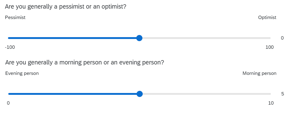
The survey also included questions asking about whether people perceive themselves as pessimists vs optimists (the outlook variable), and as an “evening person” vs a “morning person” (the ampm variable).

Fill in the blanks in this description.

A total sample of (1)______ participants completed the survey.

In their general outlook on life (measured with (2)______), participants reported an average score of (3)______ ((4)______), indicating a (5)______ disposition overall.

For chronotype — as measured on a sliding scale from 0 (“evening person”) to 10 (“morning person”) — the distribution was (6)______. Consequently, the central tendency for chronotype is best described by the (7)______ of (8)______ ((9)______), with scores ranging from (10)______ to (11)______.

TipHints

1. how many people are there in the data? (check back to week 2, or the Read in and inspect data flashcard)
2. give a brief explanation of how the optimism/pessimism was measured. Otherwise the reader won’t really know what any of the numbers mean!
3. calculate an appropriate measure of central tendency for the outlook variable.
4. calculate an appropriate measure of dispersion for the outlook variable.
5. what do 3 & 4 tell you about the sample?
   
6. describe the shape of the distribution of the ampm variable (you’ll need to plot it!)
7. what metric is best for characterising the central tendency of the ampm variable
8. calculate an appropriate measure of central tendency for the ampm variable.
9. calculate an appropriate measure of dispersion for the ampm variable.
10. calculate the minimum of the ampm variable.
11. calculate the maximum of the ampm variable.

Solution 5. A total sample of 134 participants completed the survey.

In their general outlook on life (measured with a sliding scale from -100 to 100, with ‘Pessimist’ and ‘Optimist’ at the extreme labels), participants reported an average score of 21.83 (SD = 45.86), indicating a slightly optimistic disposition overall.

For chronotype — as measured by a sliding scale from 0 (“evening person”) to 10 (“morning person”) — the distribution was (6) positively skewed . Consequently, the central tendency for chronotype is best described by the (7) median of (8) 2.75 ((9) IQR = 3.9), with scores along the entire range from 0 to 10.

Finishing up

Once you’ve finished, don’t forget to:

1. Save your R script
2. Post the R script to the group discussion space on Learn, to ensure that everyone has access to it! (For step-by-step instructions on how to do this, click here)