In this final week we are going to address some practical issues that commonly arise in Structural Equation Modeling: Non-normality, ordinal-categorical endogenous variables, and missingness. After that, we’re going to look briefly into how to simulate data based on a structural equation model.
Practical issues in SEM
One of the key assumptions of the models we have been fitting so far is that our variables are all normally distributed, and are continuous. Why?
Recall how we first introduced the idea of estimating a SEM: comparing the observed covariance matrix with our model implied covariance matrix. This heavily relies on the assumption that our observed covariance matrix provides a good representation of our data - i.e., that \(var(x_i)\) and \(cov(x_i,x_j)\) are adequate representations of the relations between variables.
Unfortunately, this is true if we have a “multivariate normal distribution”, but becomes more difficult when our variables are either not continuous or not normally distributed.
Multivariate Normal Distribution (MVN)
The multivariate normal distribution is fundamentally just the extension of our univariate normal (the bell-shaped curve we are used to seeing) to more dimensions. The condition which needs to be met is that every linear combination of the \(k\) variables has a univariate normal distribution. It is denoted by \(N(\boldsymbol{\mu}, \boldsymbol{\Sigma})\) (note that the bold font indicates that \(\boldsymbol{\mu}\) and \(\boldsymbol{\Sigma}\) are, respectively, a vector of means and a matrix of covariances).
The idea of the multivariate normal can be a bit difficult to get to grips with in part because there’s not an intuitive way to visualise it once we move beyond 2 or 3 variables.
You may also see this represented by a contour plot, which should look similar to the above 3D plot viewed from above.
Optional: covariance matrix fails to capture non-normality
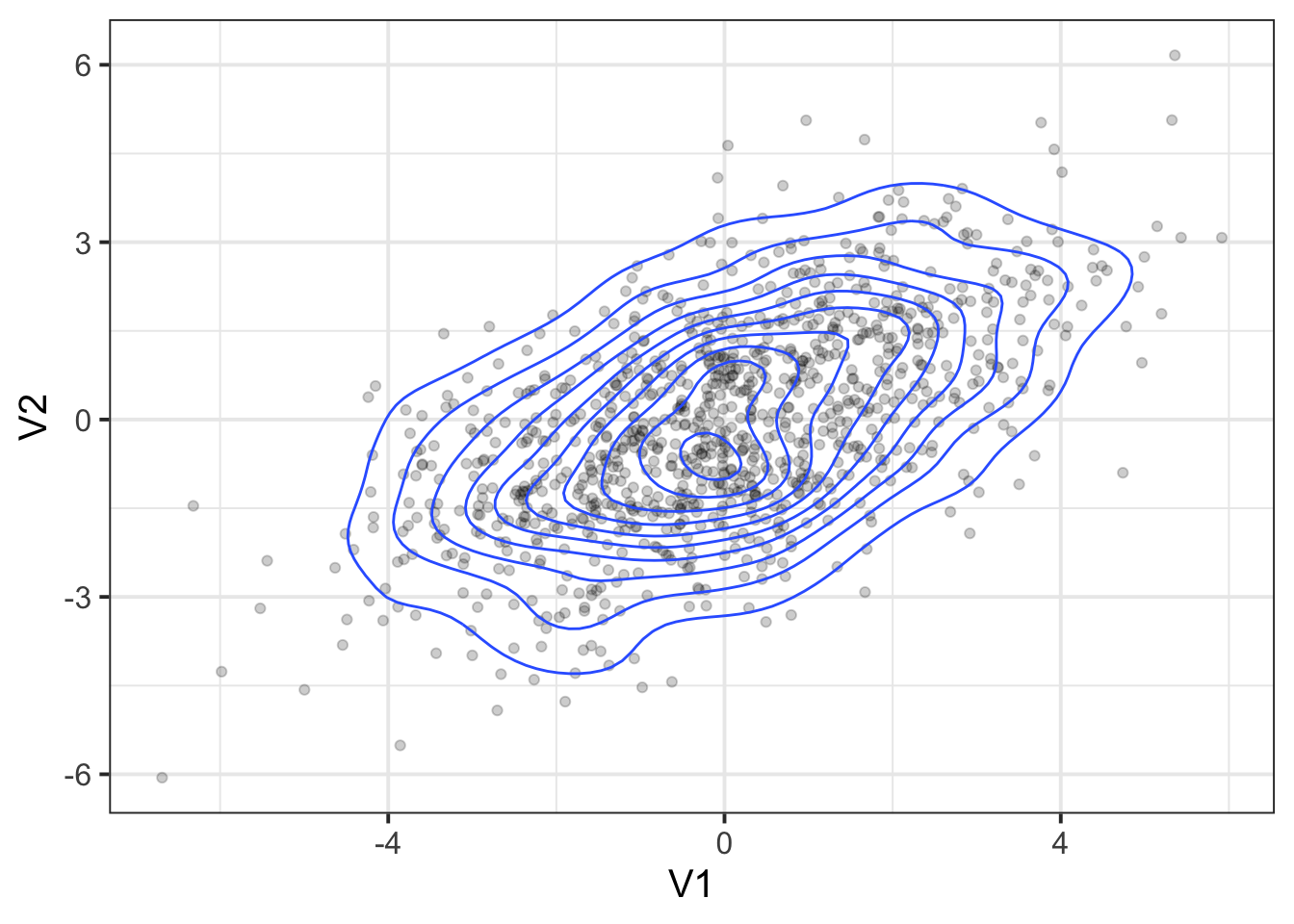
Suppose we had the following variables:
The joint probability distribution of these two variables can be visualised in Figure
2.
If we compute our covariance matrix from these variables, we get:
##       V1    V2
## V1 13.56 -5.11
## V2 -5.11  7.35
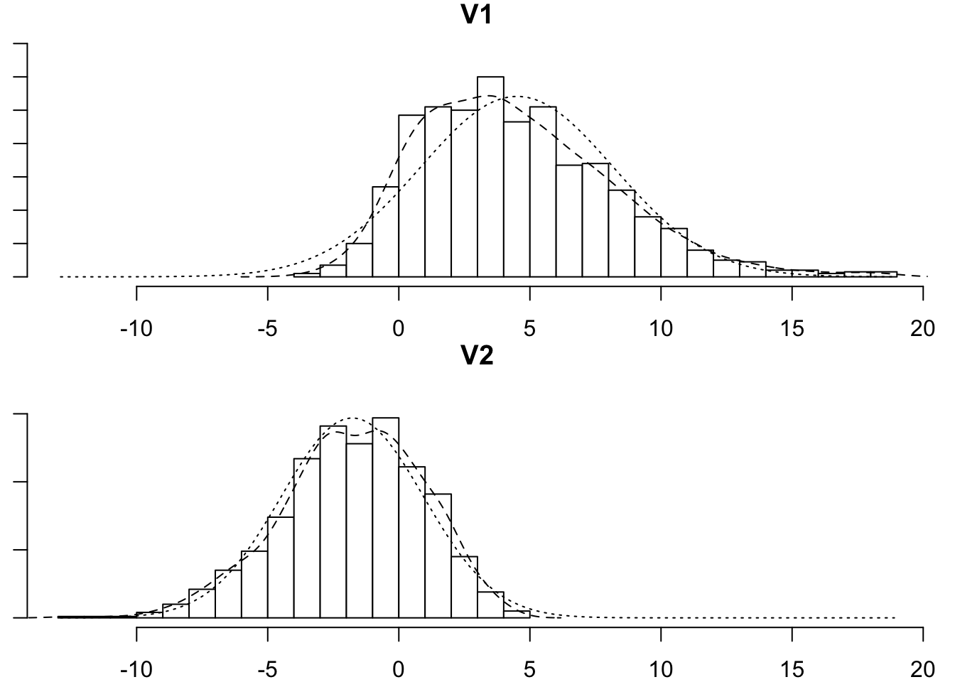
But this fails to capture information about important properties of the data relating to features such as skew (lop-sided-ness) and kurtosis (pointiness). If we simulate data based on this covariance matrix, we get something like the below, which is clearly limited in its reflection of our actual data.
Prenatal Stress & IQ data
A researcher is interested in the effects of prenatal stress on child cognitive outcomes.
She has a 5-item measure of prenatal stress and a 5 subtest measure of child cognitive ability, collected for 500 mother-infant dyads.
Question A1
Before we do anything with the data, grab some paper and sketch out the full model that you plan to fit to address the researcher’s question.
Tip: everything you need is in the description of the data. Start by drawing the specific path(s) of interest. Are these between latent variables? If so, add in the paths to the observed variables for each latent variable.
Solution
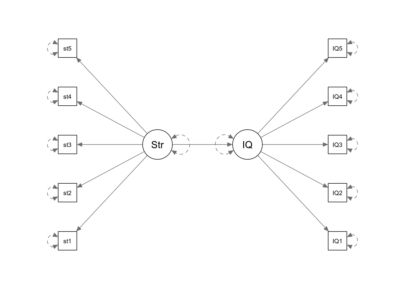
The main parameter of interest here is “the effects of prenatal stress on child cognitive outcomes”. So we have an arrow going from Stress to IQ.
Each of these are latent variables, for which we have observed 5 indicator variables, so we have an arrow going from “IQ” to each of the 5 IQ items, and from “Stress” to the 5 stress items.
Question A2
Okay, let’s get into the data then.
Read in the data and explore it.
You may remember the pairs.panels() function from the psych package. Another useful one from the same package is multi.hist().
Pay attention to the scales on which the items are measured.
Solution
Notice that the prenatal stress questionnaire items are measured on a 3-point scale.
library(tidyverse)
library(psych)

stress_IQ_data <- read_csv("https://uoepsy.github.io/data/stressIQ.csv")

describe(stress_IQ_data) # from psych package
## vars n mean sd median trimmed mad min max range skew
## ID 1 500 250.50 144.48 250.50 250.50 185.32 1.00 500.00 499.00 0.00
## stress1 2 500 1.59 0.56 2.00 1.57 0.00 1.00 3.00 2.00 0.22
## stress2 3 500 1.90 0.51 2.00 1.90 0.00 1.00 3.00 2.00 -0.16
## stress3 4 500 1.24 0.43 1.00 1.18 0.00 1.00 3.00 2.00 1.26
## stress4 5 500 2.03 0.33 2.00 2.00 0.00 1.00 3.00 2.00 0.57
## stress5 6 500 1.63 0.55 2.00 1.61 0.00 1.00 3.00 2.00 0.10
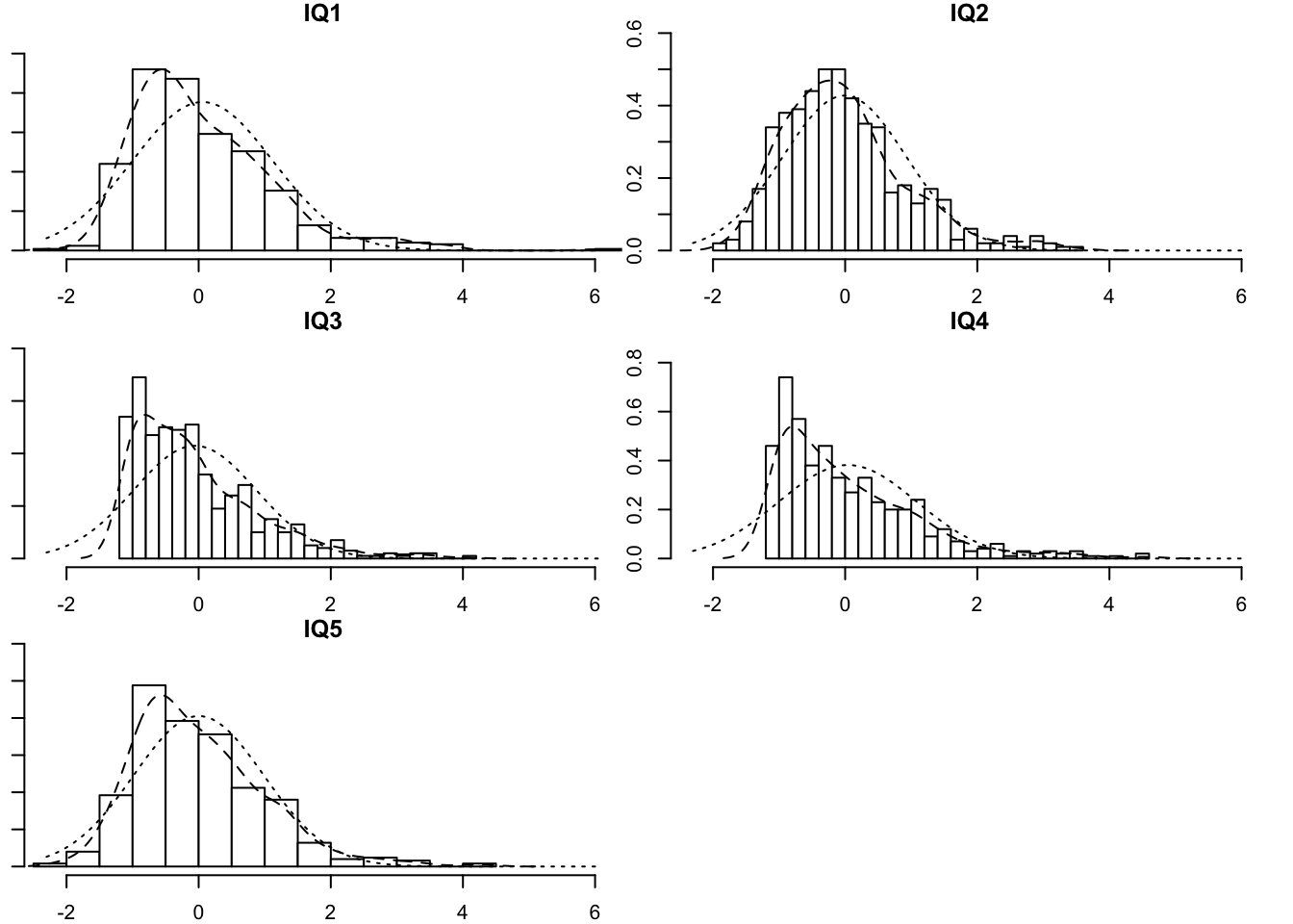
## IQ1 7 500 0.06 1.06 -0.18 -0.06 0.94 -2.25 6.02 8.28 1.28
## IQ2 8 500 -0.01 0.93 -0.13 -0.09 0.83 -1.83 3.58 5.40 0.93
## IQ3 9 500 -0.06 0.93 -0.28 -0.19 0.85 -1.07 4.05 5.12 1.34
## IQ4 10 500 0.04 1.04 -0.24 -0.11 0.94 -1.07 4.56 5.63 1.40
## IQ5 11 500 0.00 0.98 -0.16 -0.08 0.91 -2.14 4.35 6.48 0.95
## kurtosis se
## ID -1.21 6.46
## stress1 -0.90 0.02
## stress2 0.65 0.02
## stress3 -0.19 0.02
## stress4 5.78 0.01
## stress5 -0.87 0.02
## IQ1 2.72 0.05
## IQ2 1.08 0.04
## IQ3 1.93 0.04
## IQ4 2.17 0.05
## IQ5 1.39 0.04
multi.hist(stress_IQ_data, global = FALSE) # from psych package
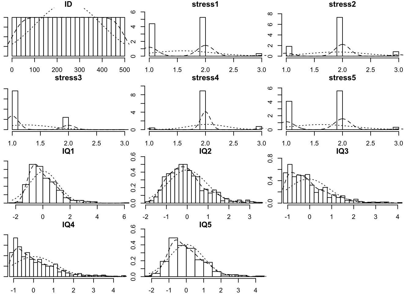
The argument global = TRUE would use the same x-axis for all histograms, and FALSE otherwise.
Ordered-Categorical Endogenous Variables
Sometimes we can treat ordinal data as if it is continuous. When exactly this is appropriate is a contentious issue - some statisticians might maintain that ordinal data is simply not continuous, so we should never treat it as such. In psychology, much research using SEM centers around questionnaire data, which lends itself to likert data (for instance, “strongly agree”,“agree”,“neither agree nor disagree”,“disagree”,“strongly disagree”). An often used rule of thumb, is that likert data with \(\geq 5\) levels can be treated as if they are continuous without unduly influencing results (see Johnson, D.R., & Creech, J.C. (1983). Ordinal measures in multiple indicator models: A simulation study of categorization error).
What we can do
In R, lavaan will automatically switch to a categorical estimator if we tell it that we have some ordered-categorical variables. We can use the ordered = c("item1name","item2name","item3name", ...) argument.
This is true for both the cfa() and sem() functions.
Question A3
The prenatal stress questionnaire items are measured on a 3-point scale.
Fit a one-factor confirmatory factor analysis for the latent factor of Stress, specifying any ordered-categorical variables in order to use an appropriate estimation method.
Solution
library(lavaan)
library(semPlot)
# specify the model
model_stress <- 'Stress =~ stress1 + stress2 + stress3 + stress4 + stress5'

# estimate the model - cfa will automatically switch to a categorical estimator if we mention that our five variables are ordered-categorical, using the 'ordered' function
model_stress.est <-
  cfa(model_stress, data=stress_IQ_data,
      ordered=c('stress1','stress2','stress3','stress4','stress5'))
Question A4
Inspect your model output. Notice that you have an extra column - we now have ‘robust’ values for the fit statistics (those that appear in the right-hand column under ‘robust’) to check that our model fits well.
Another new thing we have is the presence of ‘thresholds’ in our output. These are two thresholds per item in this example because we have a three-point response scale. Estimation of ordered-categorical variables involves constructing a hypothetical continuum underlying our categories, with “thresholds” being the points on this continuum where an observation moves from being one category to the next.
Solution
# inspect the output
summary(model_stress.est, fit.measures=T, standardized=T)
## lavaan 0.6.15 ended normally after 18 iterations
##
##   Estimator                                       DWLS
##   Optimization method                           NLMINB
##   Number of model parameters                        15
##
##   Number of observations                           500
##
## Model Test User Model:
##                                               Standard      Scaled
##   Test Statistic                                 0.520       0.773
##   Degrees of freedom                                 5           5
##   P-value (Chi-square)                           0.991       0.979
##   Scaling correction factor                                  0.740
##   Shift parameter                                            0.070
##     simple second-order correction
##
## Model Test Baseline Model:
##
##   Test statistic                               552.578     498.463
##   Degrees of freedom                                10          10
##   P-value                                        0.000       0.000
##   Scaling correction factor                                  1.111
##
## User Model versus Baseline Model:
##
##   Comparative Fit Index (CFI)                    1.000       1.000
##   Tucker-Lewis Index (TLI)                       1.017       1.017
##
##   Robust Comparative Fit Index (CFI)                         1.000
##   Robust Tucker-Lewis Index (TLI)                            1.065
##
## Root Mean Square Error of Approximation:
##
##   RMSEA                                          0.000       0.000
##   90 Percent confidence interval - lower         0.000       0.000
##   90 Percent confidence interval - upper         0.000       0.000
##   P-value H_0: RMSEA <= 0.050                    1.000       0.999
##   P-value H_0: RMSEA >= 0.080                    0.000       0.000
##
##   Robust RMSEA                                               0.000
##   90 Percent confidence interval - lower                     0.000
##   90 Percent confidence interval - upper                     0.000
##   P-value H_0: Robust RMSEA <= 0.050                         0.990
##   P-value H_0: Robust RMSEA >= 0.080                         0.004
##
## Standardized Root Mean Square Residual:
##
##   SRMR                                           0.012       0.012
##
## Parameter Estimates:
##
##   Standard errors                           Robust.sem
##   Information                                 Expected
##   Information saturated (h1) model        Unstructured
##
## Latent Variables:
##                    Estimate  Std.Err  z-value  P(>|z|)   Std.lv  Std.all
##   Stress =~
##     stress1           1.000                               0.619    0.619
##     stress2           1.111    0.121    9.214    0.000    0.688    0.688
##     stress3           1.182    0.137    8.614    0.000    0.732    0.732
##     stress4           1.049    0.130    8.089    0.000    0.649    0.649
##     stress5           1.134    0.129    8.790    0.000    0.702    0.702
##
## Intercepts:
##                    Estimate  Std.Err  z-value  P(>|z|)   Std.lv  Std.all
##    .stress1           0.000                               0.000    0.000
##    .stress2           0.000                               0.000    0.000
##    .stress3           0.000                               0.000    0.000
##    .stress4           0.000                               0.000    0.000
##    .stress5           0.000                               0.000    0.000
##     Stress            0.000                               0.000    0.000
##
## Thresholds:
##                    Estimate  Std.Err  z-value  P(>|z|)   Std.lv  Std.all
##     stress1|t1       -0.151    0.056   -2.680    0.007   -0.151   -0.151
##     stress1|t2        1.825    0.108   16.973    0.000    1.825    1.825
##     stress2|t1       -0.900    0.065  -13.806    0.000   -0.900   -0.900
##     stress2|t2        1.379    0.081   17.124    0.000    1.379    1.379
##     stress3|t1        0.700    0.061   11.399    0.000    0.700    0.700
##     stress3|t2        2.878    0.315    9.124    0.000    2.878    2.878
##     stress4|t1       -1.751    0.102  -17.198    0.000   -1.751   -1.751
##     stress4|t2        1.461    0.084   17.324    0.000    1.461    1.461
##     stress5|t1       -0.233    0.057   -4.107    0.000   -0.233   -0.233
##     stress5|t2        1.825    0.108   16.973    0.000    1.825    1.825
##
## Variances:
##                    Estimate  Std.Err  z-value  P(>|z|)   Std.lv  Std.all
##    .stress1           0.616                               0.616    0.616
##    .stress2           0.526                               0.526    0.526
##    .stress3           0.464                               0.464    0.464
##    .stress4           0.578                               0.578    0.578
##    .stress5           0.507                               0.507    0.507
##     Stress            0.384    0.064    6.011    0.000    1.000    1.000
##
## Scales y*:
##                    Estimate  Std.Err  z-value  P(>|z|)   Std.lv  Std.all
##     stress1           1.000                               1.000    1.000
##     stress2           1.000                               1.000    1.000
##     stress3           1.000                               1.000    1.000
##     stress4           1.000                               1.000    1.000
##     stress5           1.000                               1.000    1.000
Non-normality
For determining what consititutes deviations from normality, there are various measures of both skewness and kurtosis (see Joanes, D.N. and Gill, C.A (1998). Comparing measures of sample skewness and kurtosis if you’re interested). In addition, there are various suggested rules of thumb we can follow. Below are the most common:
Skewness rules of thumb:
- \(|skew| < 0.5\): fairly symmetrical
- \(0.5 < |skew| < 1\): moderately skewed
- \(1 < |skew|\): highly skewed
Kurtosis rule of thumb:
- \(Kurtosis > 3\): Heavier tails than the normal distribution. Possibly problematic
What we can do
When faced with variables which appear to deviate from normality, we should ideally use a robust estimator that corrects for any bias in the standard errors induced by non-normality, while also providing a corrected \(\chi^2\) statistic to more accurately capture the misfit of our model.
There are a few robust estimators in lavaan, but one of the more frequently used ones is “MLR” (maximum likelihood with robust SEs). You can find all the other options at https://lavaan.ugent.be/tutorial/est.html.
We can make use of these with: sem(model, estimator="MLR") or cfa(model, estimator="MLR").
Question A5
We’re now going to conduct a CFA for the IQ items.
Check their distributions (both numerically and visually) and fit a one-factor CFA using an appropriate estimation method.
Tip: the describe() function from the psych package will give you measures of skew and kurtosis.
Solution
We should check the item distributions for evidence of non-normality (skewness and kurtosis). We can use the describe() function from psych and plot the data using histograms or density curves.
library(kableExtra)

# this is just describe() but dressed up to make a nice table output (the one we see below)
stress_IQ_data %>%
    select(contains("IQ")) %>%
    describe %>%
    as.data.frame() %>%
    rownames_to_column(., var = "variable") %>%
    select(variable,mean,sd,skew,kurtosis) %>%
    kable(digits = 2) %>%
    kable_styling(full_width = FALSE)
|
variable
|
mean
|
sd
|
skew
|
kurtosis
|
|
IQ1
|
0.06
|
1.06
|
1.28
|
2.72
|
|
IQ2
|
-0.01
|
0.93
|
0.93
|
1.08
|
|
IQ3
|
-0.06
|
0.93
|
1.34
|
1.93
|
|
IQ4
|
0.04
|
1.04
|
1.40
|
2.17
|
|
IQ5
|
0.00
|
0.98
|
0.95
|
1.39
|
It looks like some of our IQ items are pretty skewed. Let’s plot them.
stress_IQ_data %>%
  select(contains("IQ")) %>%
  multi.hist
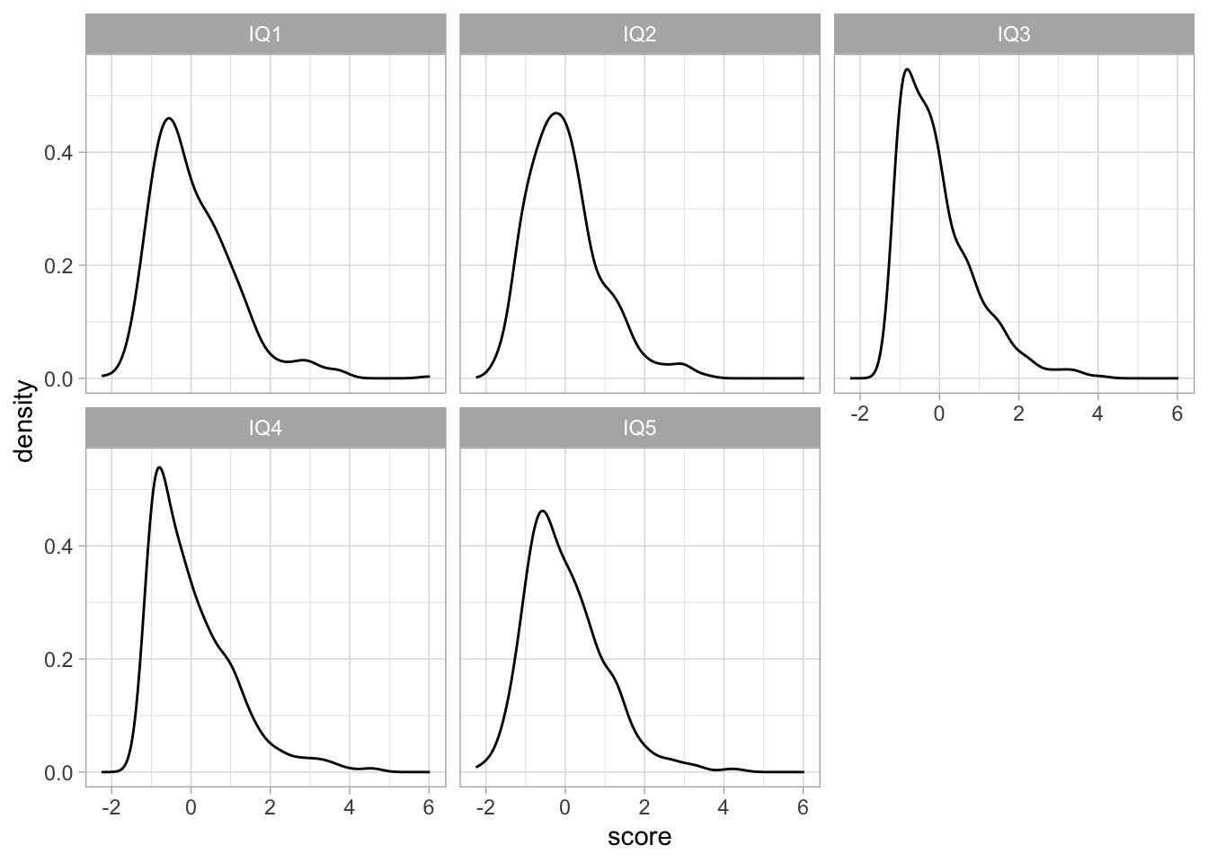
If you want a ggplot way:
## GGPLOT
# temporarily reshape the data to long format to make it quicker to plot
stress_IQ_data %>%
  pivot_longer(IQ1:IQ5, names_to="variable",values_to="score") %>%
  ggplot(aes(x=score))+
  geom_density()+
  facet_wrap(~variable)+
  theme_light()
Because our variables seem to be non-normal, therefore, we should use a robust estimator such as MLR for our CFA
model_IQ <- 'IQ =~ IQ1 + IQ2 + IQ3 + IQ4 + IQ5'

model_IQ.est <- cfa(model_IQ, data=stress_IQ_data, estimator='MLR')
Question A6
Examine the fit of the CFA model.
If it doesn’t fit very well, consider checking for areas of local misfit (i.e., check your modindices()), and adjust your model accordingly.
Solution
summary(model_IQ.est, fit.measures=T, standardized=T)
## lavaan 0.6.15 ended normally after 17 iterations
##
##   Estimator                                         ML
##   Optimization method                           NLMINB
##   Number of model parameters                        10
##
##   Number of observations                           500
##
## Model Test User Model:
##                                               Standard      Scaled
##   Test Statistic                                90.039      86.467
##   Degrees of freedom                                 5           5
##   P-value (Chi-square)                           0.000       0.000
##   Scaling correction factor                                  1.041
##     Yuan-Bentler correction (Mplus variant)
##
## Model Test Baseline Model:
##
##   Test statistic                               936.990     695.162
##   Degrees of freedom                                10          10
##   P-value                                        0.000       0.000
##   Scaling correction factor                                  1.348
##
## User Model versus Baseline Model:
##
##   Comparative Fit Index (CFI)                    0.908       0.881
##   Tucker-Lewis Index (TLI)                       0.817       0.762
##
##   Robust Comparative Fit Index (CFI)                         0.908
##   Robust Tucker-Lewis Index (TLI)                            0.816
##
## Loglikelihood and Information Criteria:
##
##   Loglikelihood user model (H0)              -3091.265   -3091.265
##   Scaling correction factor                                  1.797
##       for the MLR correction
##   Loglikelihood unrestricted model (H1)      -3046.246   -3046.246
##   Scaling correction factor                                  1.545
##       for the MLR correction
##
##   Akaike (AIC)                                6202.531    6202.531
##   Bayesian (BIC)                              6244.677    6244.677
##   Sample-size adjusted Bayesian (SABIC)       6212.936    6212.936
##
## Root Mean Square Error of Approximation:
##
##   RMSEA                                          0.184       0.181
##   90 Percent confidence interval - lower         0.152       0.149
##   90 Percent confidence interval - upper         0.219       0.214
##   P-value H_0: RMSEA <= 0.050                    0.000       0.000
##   P-value H_0: RMSEA >= 0.080                    1.000       1.000
##
##   Robust RMSEA                                               0.184
##   90 Percent confidence interval - lower                     0.151
##   90 Percent confidence interval - upper                     0.219
##   P-value H_0: Robust RMSEA <= 0.050                         0.000
##   P-value H_0: Robust RMSEA >= 0.080                         1.000
##
## Standardized Root Mean Square Residual:
##
##   SRMR                                           0.057       0.057
##
## Parameter Estimates:
##
##   Standard errors                             Sandwich
##   Information bread                           Observed
##   Observed information based on                Hessian
##
## Latent Variables:
##                    Estimate  Std.Err  z-value  P(>|z|)   Std.lv  Std.all
##   IQ =~
##     IQ1               1.000                               0.828    0.783
##     IQ2               0.856    0.048   17.840    0.000    0.709    0.761
##     IQ3               0.713    0.076    9.369    0.000    0.590    0.636
##     IQ4               0.829    0.095    8.702    0.000    0.686    0.657
##     IQ5               0.812    0.085    9.553    0.000    0.672    0.684
##
## Variances:
##                    Estimate  Std.Err  z-value  P(>|z|)   Std.lv  Std.all
##    .IQ1               0.431    0.060    7.140    0.000    0.431    0.386
##    .IQ2               0.365    0.046    7.902    0.000    0.365    0.421
##    .IQ3               0.513    0.059    8.679    0.000    0.513    0.596
##    .IQ4               0.618    0.070    8.866    0.000    0.618    0.568
##    .IQ5               0.514    0.052    9.858    0.000    0.514    0.532
##     IQ                0.686    0.097    7.044    0.000    1.000    1.000
The model doesn’t fit very well so we could check the modification indices for local mis-specifications
modindices(model_IQ.est, sort=T)
##    lhs op rhs     mi    epc sepc.lv sepc.all sepc.nox
## 12 IQ1 ~~ IQ2 82.653  0.302   0.302    0.762    0.762
## 21 IQ4 ~~ IQ5 48.799  0.224   0.224    0.397    0.397
## 17 IQ2 ~~ IQ4 29.875 -0.166  -0.166   -0.349   -0.349
## 14 IQ1 ~~ IQ4 15.906 -0.138  -0.138   -0.268   -0.268
## 15 IQ1 ~~ IQ5 15.870 -0.132  -0.132   -0.279   -0.279
## 19 IQ3 ~~ IQ4 15.720  0.122   0.122    0.216    0.216
## 18 IQ2 ~~ IQ5  6.147 -0.071  -0.071   -0.165   -0.165
## 16 IQ2 ~~ IQ3  4.216 -0.055  -0.055   -0.128   -0.128
## 13 IQ1 ~~ IQ3  3.108 -0.054  -0.054   -0.115   -0.115
## 20 IQ3 ~~ IQ5  0.305  0.016   0.016    0.031    0.031
It looks like we might need to include residual covariances between subtests 1 and 2 and between subtests 4 and 5, though if this were a real analysis we would want to double check this makes substantive sense (for example, do subtests 1 and 2 both measure memory while subtests 4 and 5 both test spatial ability?)
model2_IQ <- '
    IQ=~IQ1+IQ2+IQ3+IQ4+IQ5
    IQ1~~IQ2
    IQ4~~IQ5
'
model2_IQ.est <- cfa(model2_IQ, data=stress_IQ_data, estimator='MLR')
The fit of the model is now much improved!
summary(model2_IQ.est, fit.measures=T, standardized=T)
## lavaan 0.6.15 ended normally after 22 iterations
##
##   Estimator                                         ML
##   Optimization method                           NLMINB
##   Number of model parameters                        12
##
##   Number of observations                           500
##
## Model Test User Model:
##                                               Standard      Scaled
##   Test Statistic                                 8.709       7.422
##   Degrees of freedom                                 3           3
##   P-value (Chi-square)                           0.033       0.060
##   Scaling correction factor                                  1.173
##     Yuan-Bentler correction (Mplus variant)
##
## Model Test Baseline Model:
##
##   Test statistic                               936.990     695.162
##   Degrees of freedom                                10          10
##   P-value                                        0.000       0.000
##   Scaling correction factor                                  1.348
##
## User Model versus Baseline Model:
##
##   Comparative Fit Index (CFI)                    0.994       0.994
##   Tucker-Lewis Index (TLI)                       0.979       0.978
##
##   Robust Comparative Fit Index (CFI)                         0.994
##   Robust Tucker-Lewis Index (TLI)                            0.981
##
## Loglikelihood and Information Criteria:
##
##   Loglikelihood user model (H0)              -3050.600   -3050.600
##   Scaling correction factor                                  1.638
##       for the MLR correction
##   Loglikelihood unrestricted model (H1)      -3046.246   -3046.246
##   Scaling correction factor                                  1.545
##       for the MLR correction
##
##   Akaike (AIC)                                6125.201    6125.201
##   Bayesian (BIC)                              6175.776    6175.776
##   Sample-size adjusted Bayesian (SABIC)       6137.687    6137.687
##
## Root Mean Square Error of Approximation:
##
##   RMSEA                                          0.062       0.054
##   90 Percent confidence interval - lower         0.015       0.001
##   90 Percent confidence interval - upper         0.111       0.101
##   P-value H_0: RMSEA <= 0.050                    0.278       0.368
##   P-value H_0: RMSEA >= 0.080                    0.314       0.208
##
##   Robust RMSEA                                               0.059
##   90 Percent confidence interval - lower                     0.000
##   90 Percent confidence interval - upper                     0.114
##   P-value H_0: Robust RMSEA <= 0.050                         0.318
##   P-value H_0: Robust RMSEA >= 0.080                         0.308
##
## Standardized Root Mean Square Residual:
##
##   SRMR                                           0.017       0.017
##
## Parameter Estimates:
##
##   Standard errors                             Sandwich
##   Information bread                           Observed
##   Observed information based on                Hessian
##
## Latent Variables:
##                    Estimate  Std.Err  z-value  P(>|z|)   Std.lv  Std.all
##   IQ =~
##     IQ1               1.000                               0.724    0.685
##     IQ2               0.842    0.059   14.384    0.000    0.610    0.655
##     IQ3               0.882    0.090    9.813    0.000    0.639    0.689
##     IQ4               0.991    0.113    8.794    0.000    0.718    0.688
##     IQ5               0.935    0.096    9.751    0.000    0.677    0.689
##
## Covariances:
##                    Estimate  Std.Err  z-value  P(>|z|)   Std.lv  Std.all
##  .IQ1 ~~
##    .IQ2               0.231    0.047    4.964    0.000    0.231    0.427
##  .IQ4 ~~
##    .IQ5               0.114    0.047    2.430    0.015    0.114    0.211
##
## Variances:
##                    Estimate  Std.Err  z-value  P(>|z|)   Std.lv  Std.all
##    .IQ1               0.592    0.078    7.617    0.000    0.592    0.530
##    .IQ2               0.496    0.050    9.954    0.000    0.496    0.571
##    .IQ3               0.452    0.059    7.640    0.000    0.452    0.525
##    .IQ4               0.573    0.072    8.001    0.000    0.573    0.526
##    .IQ5               0.508    0.056    9.009    0.000    0.508    0.526
##     IQ                0.525    0.083    6.322    0.000    1.000    1.000
Question A7
Now its time to build a full SEM.
Estimate the effect of prenatal stress on IQ.
Remember: We know that IQ is non-normal, so we would like to use a robust estimator (e.g. MLR). However, as lavaan will tell you if you try using estimator="MLR", this is not supported for ordered data (i.e., the Stress items). It suggests instead using the WLSMV (weighted least square mean and variance adjusted) estimator. The WLSMV estimator is the default estimator in lavaan when ordered categorical variables are present. The WLSMV estimator is DWLS with a correction to return robust standard errors. In fact, if you notice in the output, you have a “robust” column too. Hence, you’re all good for non-normality as you have robust standard errors!
Specify and estimate your SEM model.
Solution
SEM_model <- '
    #IQ measurement model
    IQ =~ IQ1 + IQ2 + IQ3 + IQ4 + IQ5
    IQ1 ~~ IQ2
    IQ4 ~~ IQ5

    #stress measurement model
    Stress =~ stress1 + stress2 + stress3 + stress4 + stress5

    #structural part of model
    IQ ~ Stress
'
SEM_model.est <- sem(SEM_model, data=stress_IQ_data,
                     ordered=c('stress1','stress2','stress3','stress4','stress5'),
                     estimator="WLSMV")

summary(SEM_model.est, fit.measures=T, standardized=T)
## lavaan 0.6.15 ended normally after 31 iterations
##
##   Estimator                                       DWLS
##   Optimization method                           NLMINB
##   Number of model parameters                        33
##
##   Number of observations                           500
##
## Model Test User Model:
##                                               Standard      Scaled
##   Test Statistic                                16.002      27.058
##   Degrees of freedom                                32          32
##   P-value (Chi-square)                           0.992       0.715
##   Scaling correction factor                                  0.810
##   Shift parameter                                            7.300
##     simple second-order correction
##
## Model Test Baseline Model:
##
##   Test statistic                              2147.504    1242.141
##   Degrees of freedom                                45          45
##   P-value                                        0.000       0.000
##   Scaling correction factor                                  1.756
##
## User Model versus Baseline Model:
##
##   Comparative Fit Index (CFI)                    1.000       1.000
##   Tucker-Lewis Index (TLI)                       1.011       1.006
##
##   Robust Comparative Fit Index (CFI)                            NA
##   Robust Tucker-Lewis Index (TLI)                               NA
##
## Root Mean Square Error of Approximation:
##
##   RMSEA                                          0.000       0.000
##   90 Percent confidence interval - lower         0.000       0.000
##   90 Percent confidence interval - upper         0.000       0.026
##   P-value H_0: RMSEA <= 0.050                    1.000       1.000
##   P-value H_0: RMSEA >= 0.080                    0.000       0.000
##
##   Robust RMSEA                                                  NA
##   90 Percent confidence interval - lower                        NA
##   90 Percent confidence interval - upper                        NA
##   P-value H_0: Robust RMSEA <= 0.050                            NA
##   P-value H_0: Robust RMSEA >= 0.080                            NA
##
## Standardized Root Mean Square Residual:
##
##   SRMR                                           0.030       0.030
##
## Parameter Estimates:
##
##   Standard errors                           Robust.sem
##   Information                                 Expected
##   Information saturated (h1) model        Unstructured
##
## Latent Variables:
##                    Estimate  Std.Err  z-value  P(>|z|)   Std.lv  Std.all
##   IQ =~
##     IQ1               1.000                               0.714    0.676
##     IQ2               0.841    0.046   18.370    0.000    0.601    0.645
##     IQ3               0.889    0.071   12.609    0.000    0.635    0.684
##     IQ4               1.025    0.086   11.898    0.000    0.732    0.701
##     IQ5               0.961    0.077   12.402    0.000    0.686    0.698
##   Stress =~
##     stress1           1.000                               0.612    0.612
##     stress2           1.096    0.124    8.812    0.000    0.671    0.671
##     stress3           1.253    0.150    8.334    0.000    0.767    0.767
##     stress4           1.063    0.152    7.006    0.000    0.651    0.651
##     stress5           1.135    0.126    8.993    0.000    0.695    0.695
##
## Regressions:
##                    Estimate  Std.Err  z-value  P(>|z|)   Std.lv  Std.all
##   IQ ~
##     Stress            0.456    0.082    5.575    0.000    0.391    0.391
##
## Covariances:
##                    Estimate  Std.Err  z-value  P(>|z|)   Std.lv  Std.all
##  .IQ1 ~~
##    .IQ2               0.244    0.032    7.667    0.000    0.244    0.440
##  .IQ4 ~~
##    .IQ5               0.098    0.037    2.649    0.008    0.098    0.186
##
## Intercepts:
##                    Estimate  Std.Err  z-value  P(>|z|)   Std.lv  Std.all
##    .IQ1               0.059    0.059    1.013    0.311    0.059    0.056
##    .IQ2              -0.009    0.049   -0.182    0.856   -0.009   -0.010
##    .IQ3              -0.056    0.056   -0.989    0.322   -0.056   -0.060
##    .IQ4               0.040    0.064    0.620    0.535    0.040    0.038
##    .IQ5               0.001    0.051    0.017    0.987    0.001    0.001
##    .stress1           0.000                               0.000    0.000
##    .stress2           0.000                               0.000    0.000
##    .stress3           0.000                               0.000    0.000
##    .stress4           0.000                               0.000    0.000
##    .stress5           0.000                               0.000    0.000
##    .IQ                0.000                               0.000    0.000
##     Stress            0.000                               0.000    0.000
##
## Thresholds:
##                    Estimate  Std.Err  z-value  P(>|z|)   Std.lv  Std.all
##     stress1|t1       -0.151    0.056   -2.680    0.007   -0.151   -0.151
##     stress1|t2        1.825    0.108   16.973    0.000    1.825    1.825
##     stress2|t1       -0.900    0.065  -13.806    0.000   -0.900   -0.900
##     stress2|t2        1.379    0.081   17.124    0.000    1.379    1.379
##     stress3|t1        0.700    0.061   11.399    0.000    0.700    0.700
##     stress3|t2        2.878    0.315    9.124    0.000    2.878    2.878
##     stress4|t1       -1.751    0.102  -17.198    0.000   -1.751   -1.751
##     stress4|t2        1.461    0.084   17.324    0.000    1.461    1.461
##     stress5|t1       -0.233    0.057   -4.107    0.000   -0.233   -0.233
##     stress5|t2        1.825    0.108   16.973    0.000    1.825    1.825
##
## Variances:
##                    Estimate  Std.Err  z-value  P(>|z|)   Std.lv  Std.all
##    .IQ1               0.607    0.046   13.209    0.000    0.607    0.543
##    .IQ2               0.507    0.037   13.568    0.000    0.507    0.584
##    .IQ3               0.457    0.037   12.242    0.000    0.457    0.532
##    .IQ4               0.553    0.045   12.365    0.000    0.553    0.508
##    .IQ5               0.495    0.043   11.554    0.000    0.495    0.513
##    .stress1           0.625                               0.625    0.625
##    .stress2           0.550                               0.550    0.550
##    .stress3           0.411                               0.411    0.411
##    .stress4           0.576                               0.576    0.576
##    .stress5           0.517                               0.517    0.517
##    .IQ                0.432    0.053    8.205    0.000    0.847    0.847
##     Stress            0.375    0.065    5.783    0.000    1.000    1.000
##
## Scales y*:
##                    Estimate  Std.Err  z-value  P(>|z|)   Std.lv  Std.all
##     stress1           1.000                               1.000    1.000
##     stress2           1.000                               1.000    1.000
##     stress3           1.000                               1.000    1.000
##     stress4           1.000                               1.000    1.000
##     stress5           1.000                               1.000    1.000
Don’t be misled by the fact that the summary here says that the estimator is DWLS. When we have any ordered-categorical endogenous variables in the model lavaan uses DWLS (diagonally weighted least squares) estimation for the model parameters. However, because we specified it in fitting our model, WLSMV is being used to correct the standard errors.
We can see that the effect of prenatal stress on offspring IQ is \(\beta\) = 0.456 and is statistically significant at \(p<.05\).
Missing Data
Missingness
It is very common to have missing data. Participants may stop halfway through the study, may decline to be followed up (if it is longitudinal) or may simply decline to answer certain sections. In addition, missing data can occur for all sorts of technical reasons (e.g, website crash and auto-submit a questionnaire, etc.).
It is important to understand the possible reasons for missing data in order to appropriately consider what data you do have. If missing data are missing completely random, then the data you do have should still be representative of the population. But suppose you are studying cognitive decline in an aging population, and people who are suffering from cognitive impairment are less likely to attend the follow-up assessments. Is this missingness random? No. Does it affect how you should consider your available data to represent the population of interest? Yes.
There are three main explanations for missing data:
MCAR: Missing Completely At Random. Data which are MCAR are missing data for which the propensity for missingness is completely independent of any observed or unobserved variables. It is truly random if the data are missing or not.
MAR: Missing At Random. Data which are MAR are missing data for which the propensity for missingness is not random, but it can be fully explained by some variables for which there is complete data. In other words, there is a systematic relationship between missing values and observed values. For example, people who are unemployed at time of assessment will likely not respond to questions on job satisfaction. Missing values on job satisfaction is unrelated to the levels of job satisfaction, but related to their employment status.
MNAR: Missing Not At Random. Data which are MNAR are missing data for which the propensity for missingness is related to the value which is missing. For example, suppose an employer tells employees that there are a limited number of bonuses to hand out, and then employees are asked to fill out a questionnaire. Thos who are less satisfied with their job may not respond to questions on job satisfaction (if they believe it will negatively impact their chances of receiving a bonus).
To me, these are some of the most confusing terms in statistics, because “at random” is used to mean “not completely random”!?? It might be easier to think of “missing at random” as “missing conditionally at random”, but then it gives the same acronym as “completely at random”!
FIML (Full Information Maximum Likelihood)
One approach to dealing with missing data (not discussed in depth here) is imputation. This involves substituting missing values with values predicted by some model of the process which reflects the data generating process for that variable (sometimes including some stochasticity in these imputed values, sometimes not).
In SEM, there is an extremely useful method known as full information maximum likelihood (FIML) which, similar way to imputation, uses observed data to supplement missingness. Intuitively, this is a bit like using all rest of the picture to fill in the missing bits (e.g. Figure 4).
FIML utilises all observed variables (hence “full information”) to estimate missing values by maximising the likelihood of the sample as a function of the joint probability distribution of all variables. What is really neat about this is that it allows us to make full use of all our data, as it estimates missing values on all variables in our system, regardless of whether they are exogenous/endogenous variables. Compare this to functions such as lm() and lmer(), in which missing values on our explanatory variables result in simple list-wise deletion from the model. A downside, one could argue, is that you may have specific theoretical considerations about which observed variables should weigh in on estimating missingness in variable \(x\) (rather than all variables), in which case imputation techniques may be preferable.
In lavaan, we can make use of full information maximum likelihood by using missing = "FIML" in the functions cfa() and sem().
Question A8
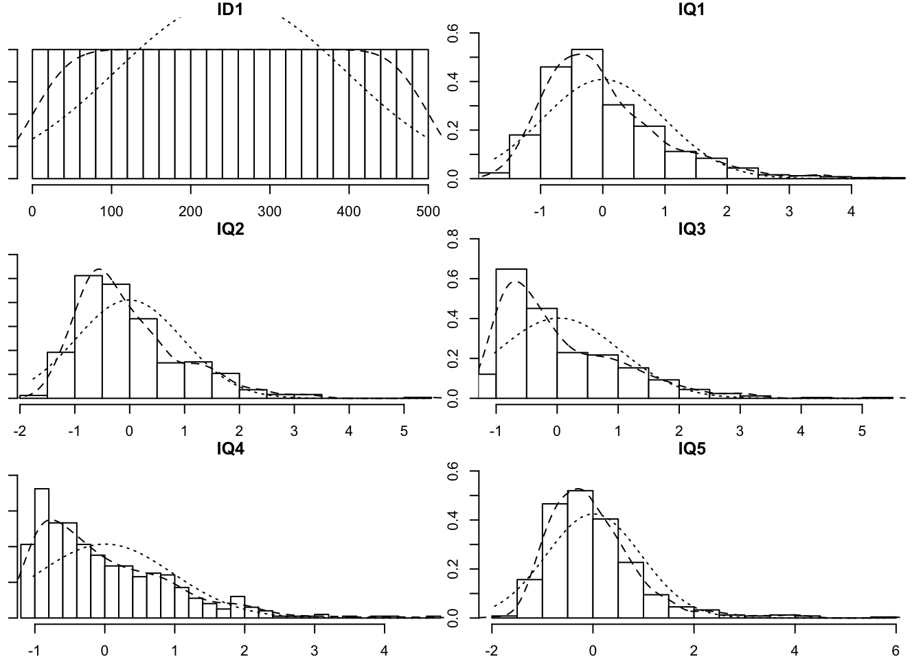
In order to try and replicate the IQ CFA, our researcher collects a new sample of size \(n=500\). However, she has some missing data (specifically, those who scored poorly on earlier tests tended to feel discouraged and chose not to complete further tests).
Read in the new dataset, plot and numerically summarise the univariate distributions of the measured variables, and then conduct a CFA using the new data, taking account of the missingness (don’t forget to also use an appropriate estimator to account for any non-normality). Does the model fit well?
Solution
We can fit the model setting missing='FIML'. If data are missing at random (MAR) - i.e., missingness is related to the measured variables but not the unobserved missing values - then this gives us unbiased parameter estimates. Unfortunately we can never know whether data are MAR for sure as this would require knowledge of the missing values.
IQ_data_new <- read_csv("https://uoepsy.github.io/data/IQdatam.csv")
multi.hist(IQ_data_new, global = FALSE)
IQ_data_new %>% select(contains("IQ")) %>%
    describe %>%
    as.data.frame() %>%
    rownames_to_column(., var = "variable") %>%
    select(variable,mean,sd,skew,kurtosis) %>%
    kable(digits = 2) %>%
    kable_styling(full_width = FALSE)
|
variable
|
mean
|
sd
|
skew
|
kurtosis
|
|
IQ1
|
0.01
|
0.98
|
1.28
|
2.29
|
|
IQ2
|
-0.01
|
0.97
|
1.25
|
2.33
|
|
IQ3
|
0.03
|
0.99
|
1.39
|
2.40
|
|
IQ4
|
0.01
|
0.96
|
1.30
|
2.05
|
|
IQ5
|
0.01
|
0.94
|
1.77
|
5.70
|
IQ_model_missing <- '
  IQ=~IQ1+IQ2+IQ3+IQ4+IQ5
  IQ1~~IQ2
  IQ4~~IQ5
'

IQ_model_missing.est <- cfa(IQ_model_missing,
                            data=IQ_data_new,
                            missing='FIML', estimator="MLR")

summary(IQ_model_missing.est, fit.measures=T, standardized=T)
## lavaan 0.6.15 ended normally after 25 iterations
##
##   Estimator                                         ML
##   Optimization method                           NLMINB
##   Number of model parameters                        17
##
##   Number of observations                           500
##   Number of missing patterns                         3
##
## Model Test User Model:
##                                               Standard      Scaled
##   Test Statistic                                 4.218       3.559
##   Degrees of freedom                                 3           3
##   P-value (Chi-square)                           0.239       0.313
##   Scaling correction factor                                  1.185
##     Yuan-Bentler correction (Mplus variant)
##
## Model Test Baseline Model:
##
##   Test statistic                               914.603     657.484
##   Degrees of freedom                                10          10
##   P-value                                        0.000       0.000
##   Scaling correction factor                                  1.391
##
## User Model versus Baseline Model:
##
##   Comparative Fit Index (CFI)                    0.999       0.999
##   Tucker-Lewis Index (TLI)                       0.996       0.997
##
##   Robust Comparative Fit Index (CFI)                         0.999
##   Robust Tucker-Lewis Index (TLI)                            0.998
##
## Loglikelihood and Information Criteria:
##
##   Loglikelihood user model (H0)              -2979.748   -2979.748
##   Scaling correction factor                                  1.635
##       for the MLR correction
##   Loglikelihood unrestricted model (H1)      -2977.639   -2977.639
##   Scaling correction factor                                  1.568
##       for the MLR correction
##
##   Akaike (AIC)                                5993.496    5993.496
##   Bayesian (BIC)                              6065.145    6065.145
##   Sample-size adjusted Bayesian (SABIC)       6011.185    6011.185
##
## Root Mean Square Error of Approximation:
##
##   RMSEA                                          0.028       0.019
##   90 Percent confidence interval - lower         0.000       0.000
##   90 Percent confidence interval - upper         0.085       0.076
##   P-value H_0: RMSEA <= 0.050                    0.658       0.756
##   P-value H_0: RMSEA >= 0.080                    0.073       0.035
##
##   Robust RMSEA                                               0.019
##   90 Percent confidence interval - lower                     0.000
##   90 Percent confidence interval - upper                     0.088
##   P-value H_0: Robust RMSEA <= 0.050                         0.682
##   P-value H_0: Robust RMSEA >= 0.080                         0.083
##
## Standardized Root Mean Square Residual:
##
##   SRMR                                           0.008       0.008
##
## Parameter Estimates:
##
##   Standard errors                             Sandwich
##   Information bread                           Observed
##   Observed information based on                Hessian
##
## Latent Variables:
##                    Estimate  Std.Err  z-value  P(>|z|)   Std.lv  Std.all
##   IQ =~
##     IQ1               1.000                               0.658    0.674
##     IQ2               0.994    0.072   13.792    0.000    0.654    0.673
##     IQ3               1.033    0.106    9.768    0.000    0.679    0.685
##     IQ4               0.989    0.113    8.788    0.000    0.651    0.676
##     IQ5               0.958    0.119    8.073    0.000    0.630    0.672
##
## Covariances:
##                    Estimate  Std.Err  z-value  P(>|z|)   Std.lv  Std.all
##  .IQ1 ~~
##    .IQ2               0.248    0.049    5.029    0.000    0.248    0.480
##  .IQ4 ~~
##    .IQ5               0.072    0.049    1.452    0.146    0.072    0.146
##
## Intercepts:
##                    Estimate  Std.Err  z-value  P(>|z|)   Std.lv  Std.all
##    .IQ1               0.010    0.044    0.229    0.819    0.010    0.010
##    .IQ2              -0.007    0.043   -0.170    0.865   -0.007   -0.008
##    .IQ3               0.027    0.044    0.602    0.547    0.027    0.027
##    .IQ4               0.002    0.043    0.050    0.960    0.002    0.002
##    .IQ5              -0.001    0.042   -0.029    0.977   -0.001   -0.001
##     IQ                0.000                               0.000    0.000
##
## Variances:
##                    Estimate  Std.Err  z-value  P(>|z|)   Std.lv  Std.all
##    .IQ1               0.519    0.064    8.103    0.000    0.519    0.545
##    .IQ2               0.515    0.063    8.222    0.000    0.515    0.546
##    .IQ3               0.521    0.063    8.324    0.000    0.521    0.530
##    .IQ4               0.504    0.062    8.190    0.000    0.504    0.543
##    .IQ5               0.482    0.069    6.998    0.000    0.482    0.549
##     IQ                0.433    0.073    5.899    0.000    1.000    1.000
Our fit indices all look very good!
Simulating Data
simulating data as an aid to learning
An extremely useful approach to learning both R and statistics is to create yourself some fake data on which you can try things out. Because you create the data, you can control any relationships, group differences etc. In doing so, you can make yourself a target to aim for.
Many of you will currently be in the process of collecting/acquiring data for your thesis. If you are yet to obtain your data, we strongly recommend that you start to simulate some data with the expected distributions in order to play around and test how your analyses works, and how to interpret the results.
For myself, I estimate that I generate fake data on average several times a week just to help me work out things I don’t understand. It also enables for easy sharing of reproducible chunks of code which can perfectly replicate issues and help discussions.
We’re going to walk through the process of fitting a structural equation model by first simulating some data.
The data simulated was generated with the following parameters (expressed in lavaan syntax). You might describe this as the “data generating process”. The goal of statistics is to shed light on the data generating process when we don’t know what it is (when we have real data).
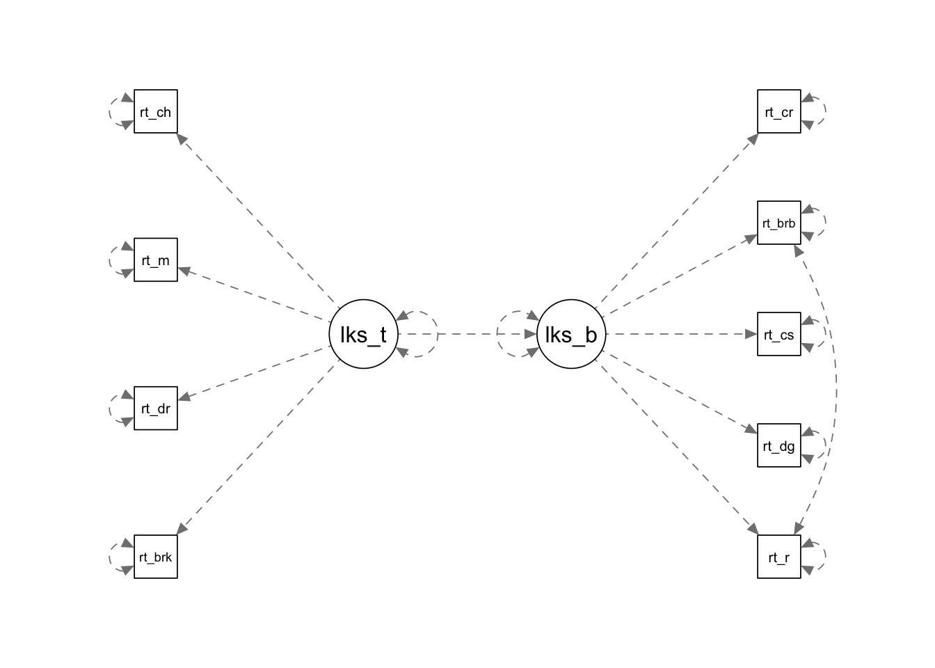
We’re going to simulate some data for which the follow model structure holds well:
likes_tea =~ rate_breakfast + rate_darjeeling + rate_mint + rate_chamomile
likes_biscuits =~ rate_oreo + rate_digestive + rate_custardcream + rate_bourbon + rate_crackers
rate_bourbon ~~ rate_oreo

likes_biscuits ~ likes_tea
As you can see, in the data generating process, there are 2 factors each measured by 4 or 5 items. Factor “likes_tea” reflects people’s enjoyment of tea, which is measured by various ratings of specific teas (these things are the things we would directly measure). The second factor is the same idea, but for biscuits.
We’ve then regressed liking biscuits onto liking tea (e.g. do people who like tea more, also like biscuits more?). Additionally, we’ve added in a covariance between ratings of oreos with ratings of bourbons, suggesting that these are related in some way beyond their representation of “liking biscuits” (perhaps this covariance is the preference for specifically chocolate flavours?).
You can find the data at https://uoepsy.github.io/data/teabiscuit.csv, or run the code below to simulate it yourself.
The lavaan package makes it really easy to simulate data, we just need to specify the magnitude of the paths, and give it to the simulateData() function.
Before simulating random data, however, it is good practice to set the random seed to ensure you will be able to reproduce your results. If you place the line set.seed(<any whole number>) at the start of your R code, every time you will run your file line by line and in order, you will get the same results.
set.seed(987)
mdl <- "
likes_tea =~ 0.9*rate_breakfast + 0.7*rate_darjeeling + 0.6*rate_mint + 0.6*rate_chamomile
likes_biscuits =~ 0.8*rate_oreo + 0.8*rate_digestive + 0.7*rate_custardcream + 0.9*rate_bourbon + 0.3*rate_crackers
rate_bourbon ~~ 0.4*rate_oreo

likes_biscuits ~ 0.3*likes_tea
"
semPaths(lavaanify(mdl),rotation=2)
df <- simulateData(mdl, sample.nobs = 300)
Question B1: Open-ended
Now that we have our data, we can try fitting models to it. Doing research with real data is like coming in at this point, and not knowing the model that was used to generate the data.
Try playing around and fitting different models to the data above, and evaluating how well they fit. What happens if you misspecify the measurement model? What happens if you leave out estimating the covariance between bourbons and oreos? Check your modification indices.