EFA and PCA
Thinking about measurement
In the second block of the MSMR course, we’re going to look at “latent variable modeling”.
Take a moment to think about the various constructs that you are interested in as a researcher. This might be anything from personality traits, to language proficiency, social identity, anxiety, etc. How we measure such constructs is a very important consideration for research. The things we’re interested in are very rarely the things we are directly measuring.
The most common way to start thinking about latent variables is to consider how we might assess levels of anxiety or depression. More often than not, we measure these using questionnaire based methods. Can we ever directly measure anxiety? 1. This inherently leads to the notion of measurement error - two people both scoring 11 on the Generalised Anxiety Disorder 7 (GAD-7) scale will not have identical levels of anxiety.
Before we start to explore how we might use a latent variable modelling approach to accommodate this idea, we’re going to start with the basic concept of reducing the dimensionality of our data.
New packages
We’re going to be needing some different packages this week (no more lme4!).
Make sure you have these packages installed:
- psych
- GPArotation
- car
Principal component analysis (PCA)
The goal of principal component analysis (PCA) is to find a smaller number of uncorrelated variables which are linear combinations of the original (many) variables and explain most of the variation in the data.
Data: Job Performance
The file job_performance.csv (available at https://uoepsy.github.io/data/job_performance.csv) contains data on fifty police officers who were rated in six different categories as part of an HR procedure. The rated skills were:
- communication skills:
commun - problem solving:
probl_solv - logical ability:
logical - learning ability:
learn - physical ability:
physical - appearance:
appearance
Load the job performance data into R and call it job.
Check whether or not the data were read correctly into R - do the dimensions correspond to the description of the data above?
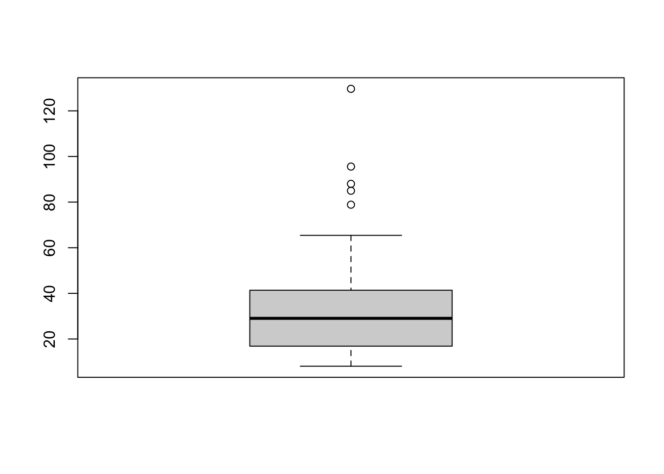
Provide descriptive statistics for each variable in the dataset.
Preliminaries
Is PCA needed?
If the original variables are highly correlated, it is possible to reduce the dimensionality of the problem under investigation without losing too much information.
On the other side, when the correlation between the variables under study is weak, a larger number of components is needed in order to explain sufficient variability.
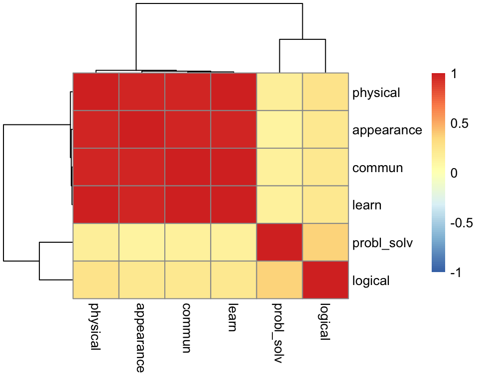
Investigate whether or not the recorded variables are highly correlated and explain whether or not you PCA might be useful in this case.
Hint: We only have 6 variables here, but if we had many, how might you visualise cor(job)?
Cov vs Cor
Should we perform PCA on the covariance or the correlation matrix?
This depends on the variances of the variables in the dataset. If the variables have large differences in their variances, then the variables with the largest variances will tend to dominate the first few principal components.
A solution to this is to standardise the variables prior to computing the covariance matrix - i.e., compute the correlation matrix!
# show that the correlation matrix and the covariance matrix of the standardized variables are identical
all.equal(cor(job), cov(scale(job)))
## [1] TRUELook at the variance of the variables in the data set. Do you think that PCA should be carried on the covariance matrix or the correlation matrix?
Perform PCA
Using the principal() function from the psych package, we can perform a PCA of the job performance data, Call the output job_pca.
job_pca <- principal(job, nfactors = ncol(job), covar = ..., rotate = 'none')
job_pca$loadings
Depending on your answer to the previous question, either set covar = TRUE or covar = FALSE within the principal() function.
Warning: the output of the function will be in terms of standardized variables nevertheless. So you will see output with standard deviation of 1.
The output
job_pca$loadings##
## Loadings:
## PC1 PC2 PC3 PC4 PC5 PC6
## commun 0.984 -0.120 0.101
## probl_solv 0.223 0.810 0.543
## logical 0.329 0.747 -0.578
## learn 0.987 -0.110 0.105
## physical 0.988 -0.110
## appearance 0.979 -0.125 0.161
##
## PC1 PC2 PC3 PC4 PC5 PC6
## SS loadings 4.035 1.261 0.631 0.035 0.022 0.016
## Proportion Var 0.673 0.210 0.105 0.006 0.004 0.003
## Cumulative Var 0.673 0.883 0.988 0.994 0.997 1.000The output is made up of two parts.
First, it shows the loading matrix. In each column of the loading matrix we find how much each of the measured variables contributes to the computed new axis/direction (that is, the principal component). Notice that there are as many principal components as variables.
The second part of the output displays the contribution of each component to the total variance.
Before interpreting it however, let’s focus on the last row of that output called “Cumulative Var”. This displays the cumulative sum of the variances of each principal component. Taken all together, the six principal components taken explain all of the total variance in the original data. In other words, the total variance of the principal components (the sum of their variances) is equal to the total variance in the original data (the sum of the variances of the variables).
However, our goal is to reduce the dimensionality of our data, so it comes natural to wonder which of the six principal components explain most of the variability, and which components instead do not contribute substantially to the total variance.
To that end, the second row “Proportion Var” displays the proportion of the total variance explained by each component, i.e. the variance of the principal component divided by the total variance.
The last row, as we saw, is the cumulative proportion of explained variance: 0.673, 0.673 + 0.210, 0.673 + 0.210 + 0.105, and so on.
We also notice that the first PC alone explains 67.3% of the total variability, while the first two components together explain almost 90% of the total variability. From the third component onwards, we do not see such a sharp increase in the proportion of explained variance, and the cumulative proportion slowly reaches the total ratio of 1 (or 100%).
How many components to keep?
There is no single best method to select the optimal number of components to keep, while discarding the remaining ones (which are then considered as noise components).
The following three heuristic rules are commonly used in the literature:
- The cumulative proportion of explained variance criterion
- Kaiser’s rule
- The scree plot
- Velicer’s Minimum Average Partial method
- Parallel analysis
In the next sections we will analyse each of them in turn.
The cumulative proportion of explained variance criterion
The rule suggests to keep as many principal components as needed in order to explain approximately 80-90% of the total variance.
Looking again at the PCA output, how many principal components would you keep if you were following the cumulative proportion of explained variance criterion?
Kaiser’s rule
According to Kaiser’s rule, we should keep the principal components having variance larger than 1. Standardized variables have a variance equal 1. Because we have 6 variables in the data set, and the total variance is 6, the value 1 represents the average variance in the data: \[ \frac{1 + 1 + 1 + 1 + 1 + 1}{6} = 1 \]
Hint:
The variances of each PC are shown in the row of the output named SS loadings and also in
job_pca$values. The average variance is:
mean(job_pca$values)## [1] 1Looking again at the PCA output, how many principal components would you keep if you were following Kaiser’s criterion?
The scree plot
The scree plot is a graphical criterion which involves plotting the variance for each principal component.
This can be easily done by calling plot on the variances, which are stored in job_pca$values
plot(x = 1:length(job_pca$values), y = job_pca$values,
     type = 'b', xlab = '', ylab = 'Variance',
     main = 'Police officers: scree plot', frame.plot = FALSE)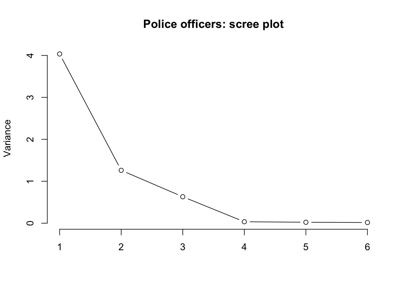
where the argument type = 'b' tells R that the plot should have both points and lines.
A typical scree plot features higher variances for the initial components and quickly drops to small variances where the curve is almost flat. The flat part of the curve represents the noise components, which are not able to capture the main sources of variability in the system.
The “elbow” in a scree plot is where the eigenvalues seem almost flat. According to the scree plot criterion, we should retain the components to the left of the “elbow” point.
Alternatively, some people prefer to use the function scree() from the psych package:
scree(job, factors = FALSE)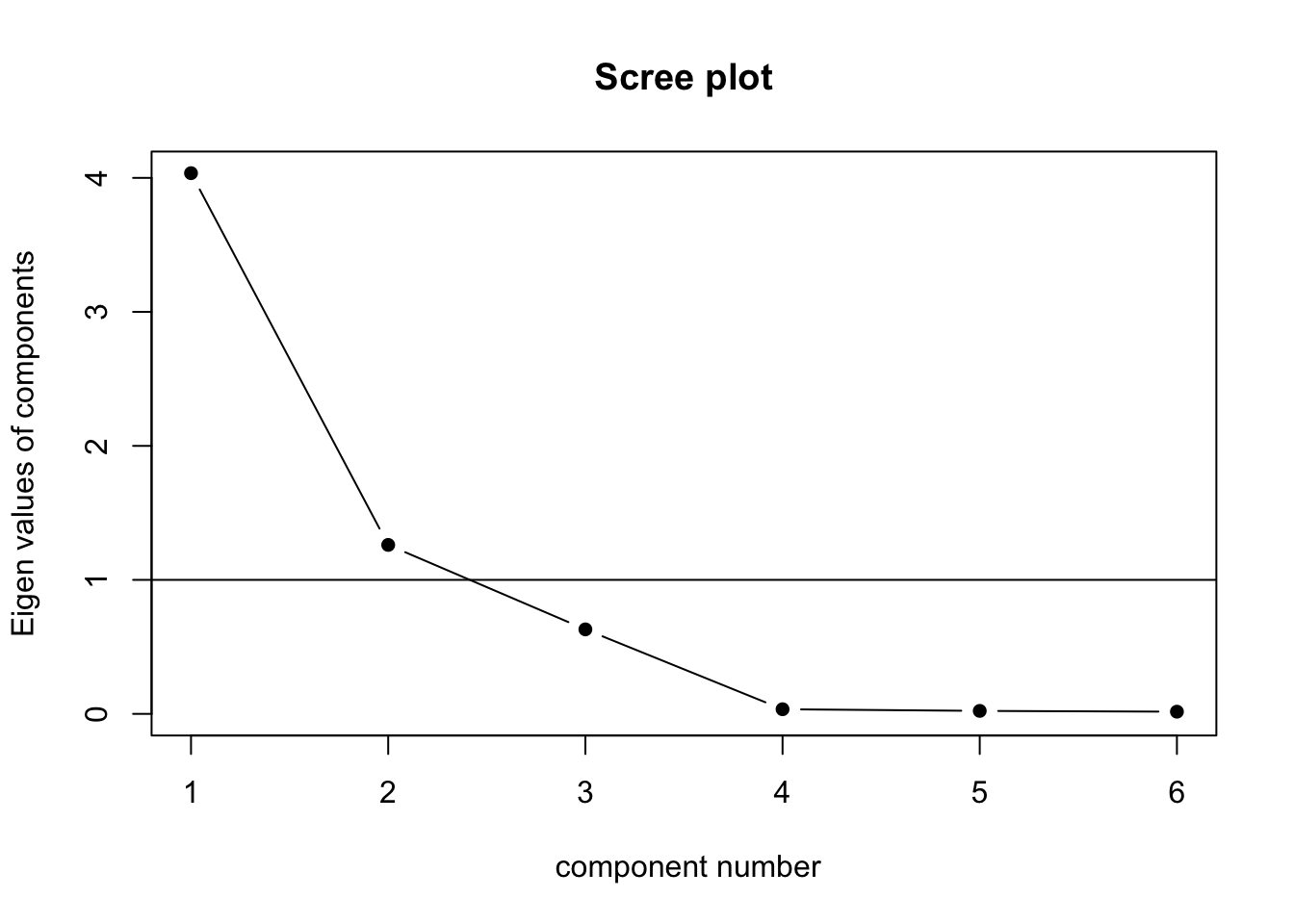
This also draws a horizontal line at y = 1. So, if you are making a decision about how many PCs to keep by looking at where the plot falls below the y = 1 line, you are basically following Kaiser’s rule. In fact, Kaiser’s criterion tells you to keep as many PCs as are those with a variance (= eigenvalue) greater than 1.
According to the scree plot, how many principal components would you retain?
Velicer’s Minimum Average Partial method
The Minimum Average Partial (MAP) test computes the partial correlation matrix (removing and adjusting for a component from the correlation matrix), sequentially partialling out each component. At each step, the partial correlations are squared and their average is computed.
At first, the components which are removed will be those that are most representative of the shared variance between 2+ variables, meaning that the “average squared partial correlation” will decrease. At some point in the process, the components being removed will begin represent variance that is specific to individual variables, meaning that the average squared partial correlation will increase.
The MAP method is to keep the number of components for which the average squared partial correlation is at the minimum.
We can conduct MAP in R using:
VSS(data, plot = FALSE, method="pc", n = ncol(data))(be aware there is a lot of other information in this output too! For now just focus on the map column)
How many components should we keep according to the MAP method?
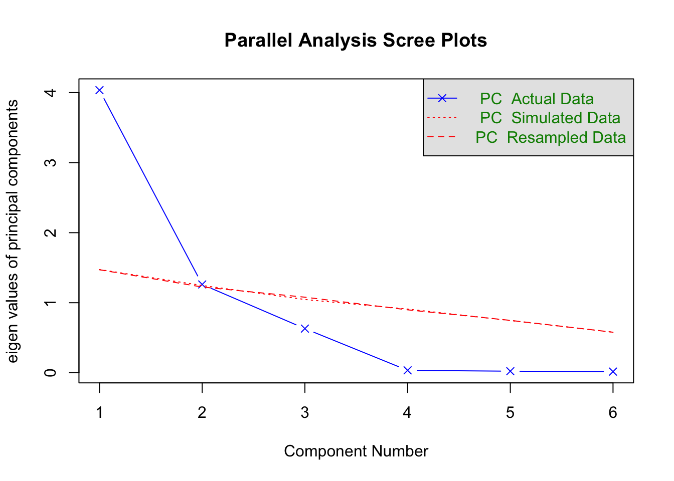
Parallel analysis
Parallel analysis involves simulating lots of datasets of the same dimension but in which the variables are uncorrelated. For each of these simulations, a PCA is conducted on its correlation matrix, and the eigenvalues are extracted. We can then compare our eigenvalues from the PCA on our actual data to the average eigenvalues across these simulations. In theory, for uncorrelated variables, no components should explain more variance than any others, and eigenvalues should be equal to 1. In reality, variables are rarely truly uncorrelated, and so there will be slight variation in the magnitude of eigenvalues simply due to chance. The parallel analysis method suggests keeping those components for which the eigenvalues are greater than those from the simulations.
It can be conducted in R using:
fa.parallel(job, fa="pc", quant=.95)How many components should we keep according to parallel analysis?
Interpretation
Because three out of the five selection criteria introduced above suggest to keep 2 principal components, in the following we will work with the first two PCs only.
Let’s have a look at the selected principal components:
job_pca$loadings[, 1:2]## PC1 PC2
## commun 0.984 -0.1197
## probl_solv 0.223 0.8095
## logical 0.329 0.7466
## learn 0.987 -0.1097
## physical 0.988 -0.0784
## appearance 0.979 -0.1253and at their corresponding proportion of total variance explained:
job_pca$values / sum(job_pca$values)## [1] 0.67253 0.21016 0.10510 0.00577 0.00372 0.00273We see that the first PC accounts for 67.3% of the total variability. All loadings seem to have the same magnitude apart from probl_solv and logical which are closer to zero.
The first component looks like a sort of average of the officers performance scores excluding problem solving and logical ability.
The second principal component, which explains only 21% of the total variance, has two loadings clearly distant from zero: the ones associated to problem solving and logical ability. It distinguishes police officers with strong logical and problem solving skills and a low score on the test (note the negative magnitude) from the other officers.
We have just seen how to interpret the first components by looking at the magnitude and sign of the coefficients for each measured variable.
For interpretation purposes, it might help hiding very small loadings. This can be done by specifying the cutoff value in the print() function. However, this only works when you pass the loadings for all the PCs:
print(job_pca$loadings, cutoff = 0.3)##
## Loadings:
## PC1 PC2 PC3 PC4 PC5 PC6
## commun 0.984
## probl_solv 0.810 0.543
## logical 0.329 0.747 -0.578
## learn 0.987
## physical 0.988
## appearance 0.979
##
## PC1 PC2 PC3 PC4 PC5 PC6
## SS loadings 4.035 1.261 0.631 0.035 0.022 0.016
## Proportion Var 0.673 0.210 0.105 0.006 0.004 0.003
## Cumulative Var 0.673 0.883 0.988 0.994 0.997 1.000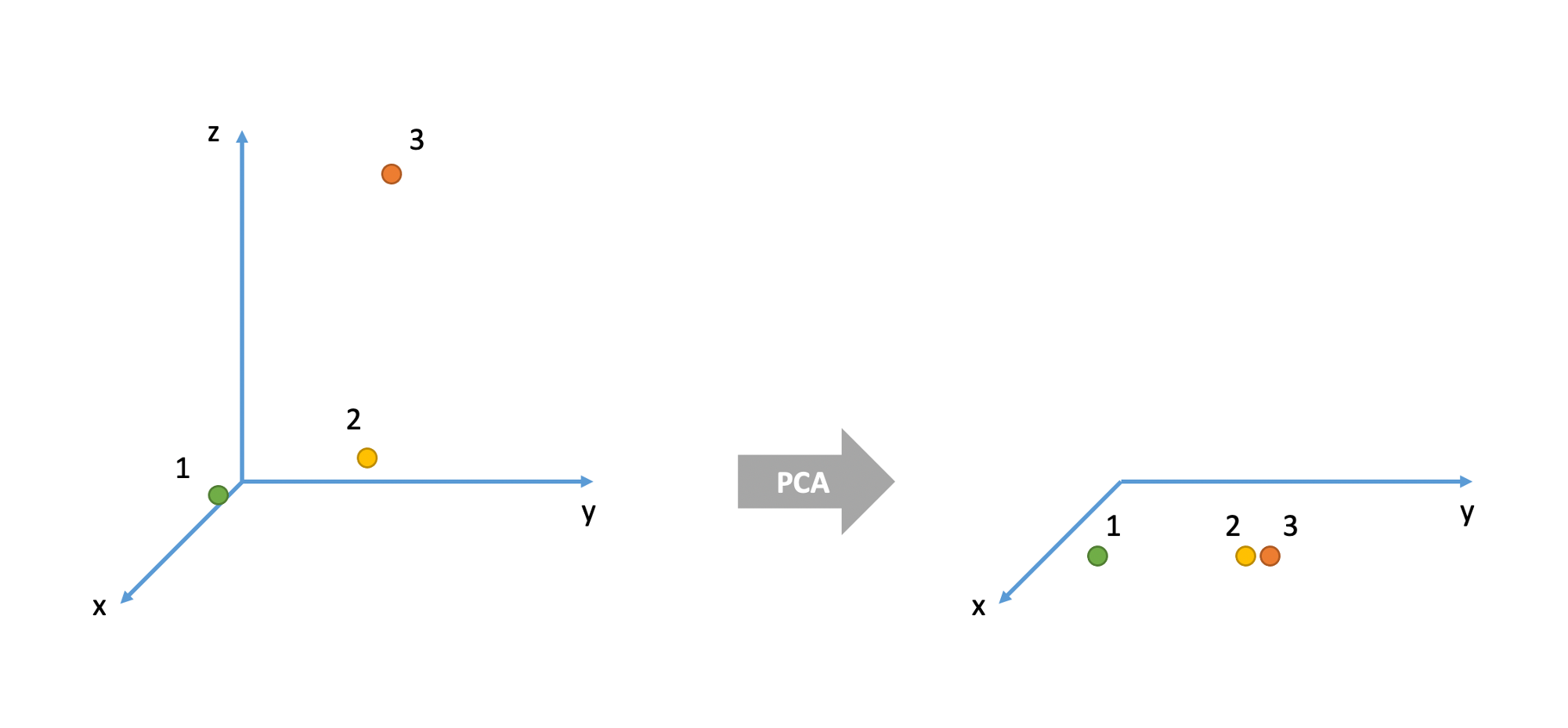
PCA scores
Supposing that we decide to reduce our six variables down to two principal components:
job_pca2 <- principal(job, nfactors = 2, covar = TRUE, rotate = 'none')We can, for each of our observations, get their scores on each of our components.
head(job_pca2$scores)## PC1 PC2
## [1,] -6.10 -1.796
## [2,] -4.69 4.164
## [3,] -5.18 -0.131
## [4,] -4.31 -1.758
## [5,] -3.71 1.207
## [6,] -3.88 -5.200In the literature, some authors also suggest to look at the correlation between each principal component and the measured variables:
# First PC
cor(job_pca2$scores[,1], job)
## commun probl_solv logical learn physical appearance
## [1,] 0.985 0.214 0.319 0.988 0.989 0.981The first PC is strongly correlated with all the measured variables except probl_solv and logical.
As we mentioned above, all variables seem to contributed to the first PC.
# Second PC
cor(job_pca2$scores[,2], job)
## commun probl_solv logical learn physical appearance
## [1,] -0.163 0.792 0.738 -0.154 -0.122 -0.169The second PC is strongly correlated with probl_solv and logical, and slightly negatively correlated with the remaining variables. This separates police offices with clear logical and problem solving skills and a small score on the test (negative sign) from the others.
We have reduced our six variables down to two principal components, and we are now able to use the scores on each component in a subsequent analysis!
For instance, if we also had information on how many arrests each police officer made, and the HR department were interested in whether the 6 questions we started with are a good predictor of this.
We could imagine conducting an analysis like the below:
# add the PCA scores to the dataset
job <-
  job %>% mutate(
    skills_score1 = job_pca2$scores[,1],
    skills_score2 = job_pca2$scores[,2]
  )
# use the scores in an analysis
lm(nr_arrests ~ skills_score1 + skills_score2, data = job)
Plotting the retained principal components
We can also visualise the statistical units (police officers) in the reduced space given by the retained principal component scores.
tibble(pc1 = job_pca$scores[, 1],
       pc2 = job_pca$scores[, 2]) %>%
  ggplot(.,aes(x=pc1,y=pc2))+
  geom_point()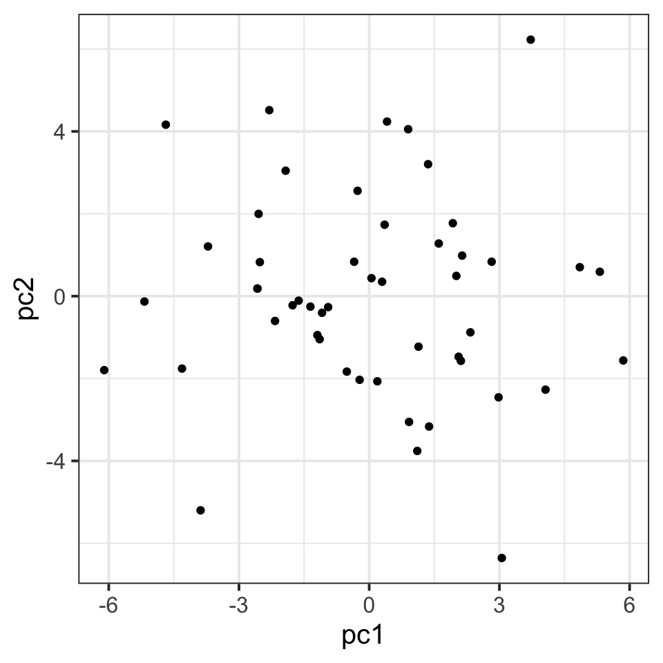
Exploratory Factor Analysis (EFA)
Where PCA aims to summarise a set of measured variables into a set of orthogonal (uncorrelated) components as linear combinations (a weighted average) of the measured variables, Factor Analysis (FA) assumes that the relationships between a set of measured variables can be explained by a number of underlying latent factors.
Note how the directions of the arrows in Figure 2 are different between PCA and FA - in PCA, each component \(C_i\) is the weighted combination of the observed variables \(y_1, ...,y_n\), whereas in FA, each measured variable \(y_i\) is seen as generated by some latent factor(s) \(F_i\) plus some unexplained variance \(u_i\).
It might help to read the \(\lambda\)s as beta-weights (\(b\), or \(\beta\)), because that’s all they really are. The equation \(y_i = \lambda_{1i}F_1 + \lambda_{2i}F_2 + u_i\) is just our way of saying that the variable \(y_i\) is the manifestation of some amount (\(\lambda_{1i}\)) of an underlying factor \(F_1\), some amount (\(\lambda_{2i}\)) of some other underlying factor \(F_2\), and some error (\(u_i\)).
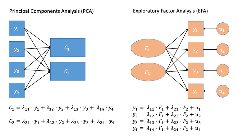
Figure 2: Path diagrams for PCA and FA
In Exploratory Factor Analysis (EFA), we are starting with no hypothesis about either the number of latent factors or about the specific relationships between latent factors and measured variables (known as the factor structure). Typically, all variables will load on all factors, and a transformation method such as a rotation (we’ll cover this in more detail below) is used to help make the results more easily interpretable.
A brief look to next week
When we have some clear hypothesis about relationships between measured variables and latent factors, we might want to impose a specific factor structure on the data (e.g., items 1 to 10 all measure social anxiety, items 11 to 15 measure health anxiety, and so on). When we impose a specific factor structure, we are doing Confirmatory Factor Analysis (CFA).
This will be the focus of next week, but it’s important to note that in practice EFA is not wholly “exploratory” (your theory will influence the decisions you make) nor is CFA wholly “confirmatory” (in which you will inevitably get tempted to explore how changing your factor structure might improve fit).
Data: Conduct Problems
A researcher is developing a new brief measure of Conduct Problems. She has collected data from n=450 adolescents on 10 items, which cover the following behaviours:
- Stealing
- Lying
- Skipping school
- Vandalism
- Breaking curfew
- Threatening others
- Bullying
- Spreading malicious rumours
- Using a weapon
- Fighting
Your task is to use the dimension reduction techniques you learned about in the lecture to help inform how to organise the items she has developed into subscales.
The data can be found at https://uoepsy.github.io/data/conduct_probs.csv
Preliminaries
Read in the dataset from https://uoepsy.github.io/data/conduct_probs.csv.
The first column is clearly an ID column, and it is easiest just to discard this when we are doing factor analysis.
Create a correlation matrix for the items.
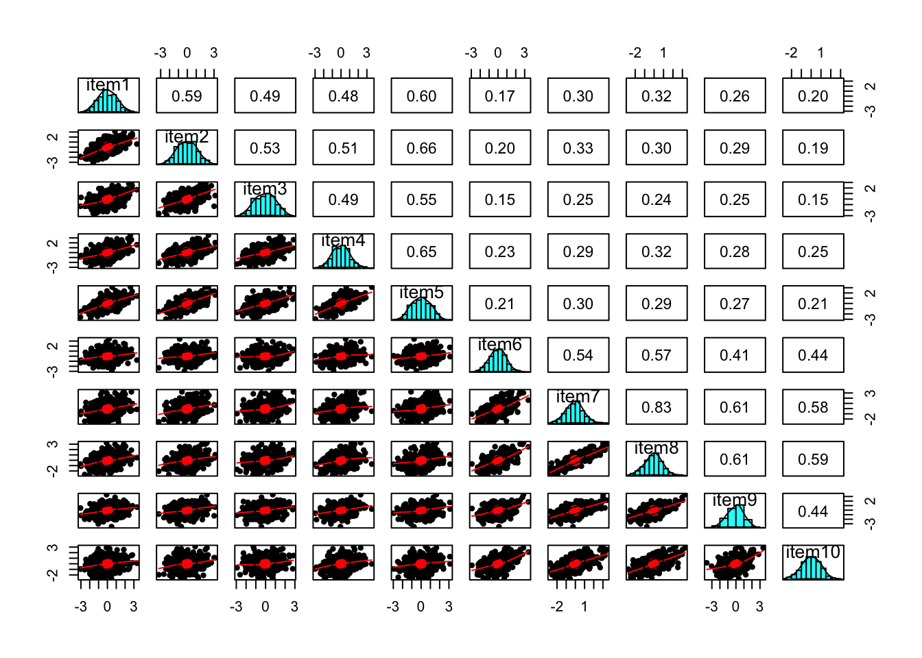
Inspect the items to check their suitability for exploratory factor analysis.
- You can use a function such as
cororcorr.test(data)(from the psych package) to create the correlation matrix.
- The function
cortest.bartlett(cor(data), n = nrow(data))conducts Bartlett’s test that the correlation matrix is proportional to the identity matrix (a matrix of all 0s except for 1s on the diagonal).
- You can check linearity of relations using
pairs.panels(data)(also from psych), and you can view the histograms on the diagonals, allowing you to check univariate normality (which is usually a good enough proxy for multivariate normality). - You can check the “factorability” of the correlation matrix using
KMO(data)(also from psych!).- Rules of thumb:
- \(0.8 < MSA < 1\): the sampling is adequate
- \(MSA <0.6\): sampling is not adequate
- \(MSA \sim 0\): large partial correlations compared to the sum of correlations. Not good for FA
- Rules of thumb:
 or alternatively, if you want a ggplot based approach:
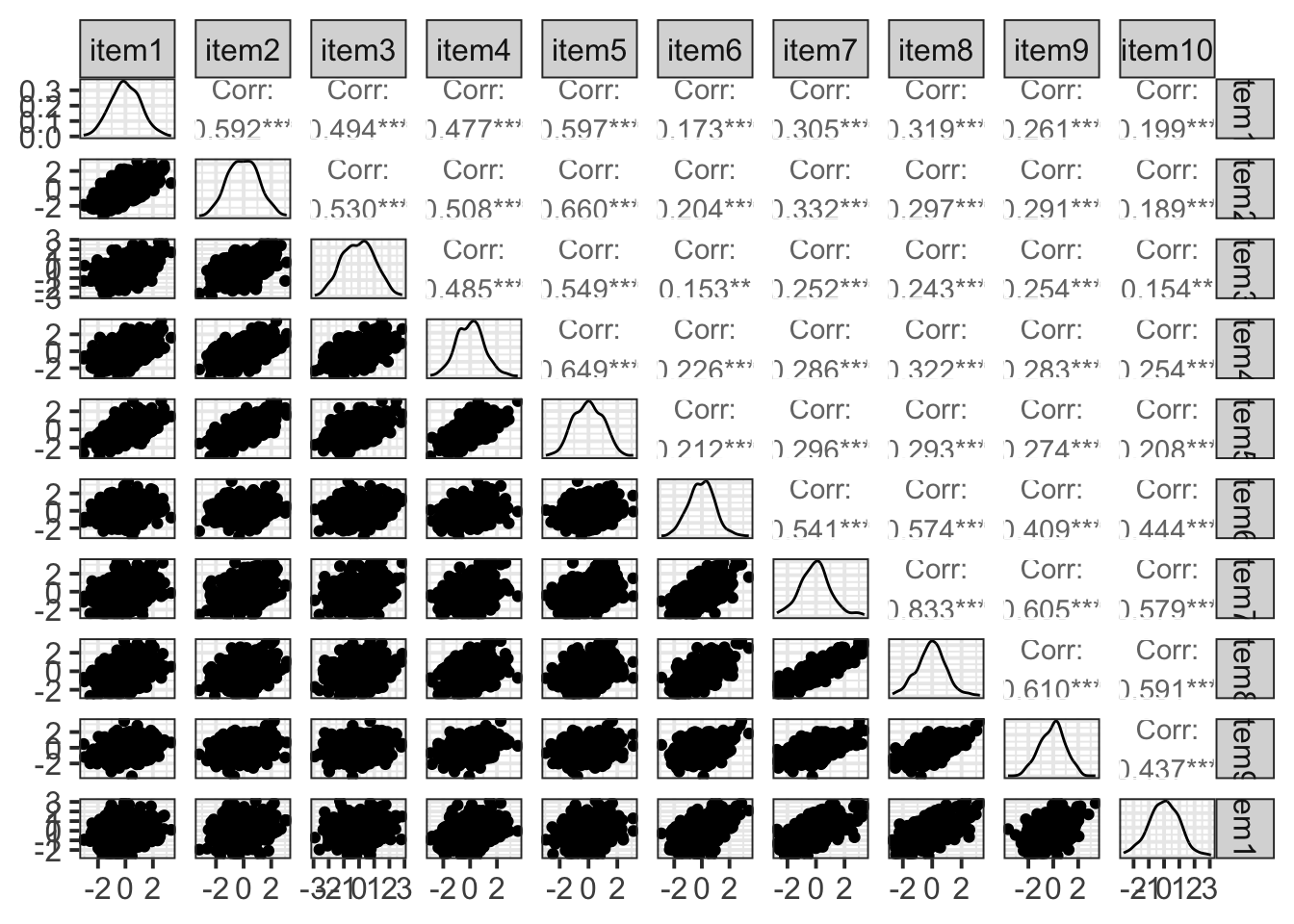
How many factors?
How many dimensions should be retained? This question can be answered in the same way as we did above for PCA.
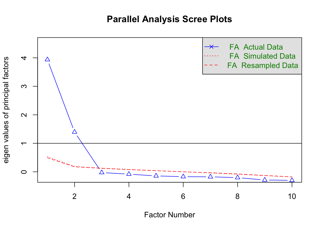
Use a scree plot, parallel analysis, and MAP test to guide you.
You can use fa.parallel(data, fm = "fa") to conduct both parallel analysis and view the scree plot!
Perform EFA
Now we need to perform the factor analysis. But there are two further things we need to consider, and they are:
- whether we want to apply a rotation to our factor loadings, in order to make them easier to interpret, and
- how do we want to extract our factors (it turns out there are loads of different approaches!).
Rotations?
Rotations are so called because they transform our loadings matrix in such a way that it can make it more easy to interpret. You can think of it as a transformation applied to our loadings in order to optimise interpretability, by maximising the loading of each item onto one factor, while minimising its loadings to others. We can do this by simple rotations, but maintaining our axes (the factors) as perpendicular (i.e., uncorrelated) as in Figure 4, or we can allow them to be transformed beyond a rotation to allow the factors to correlate (Figure 5).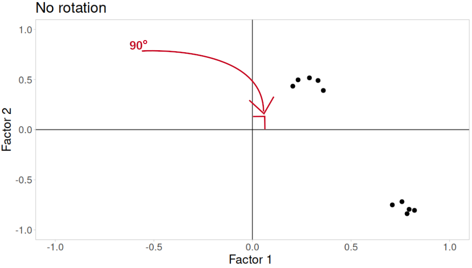
Figure 3: No rotation
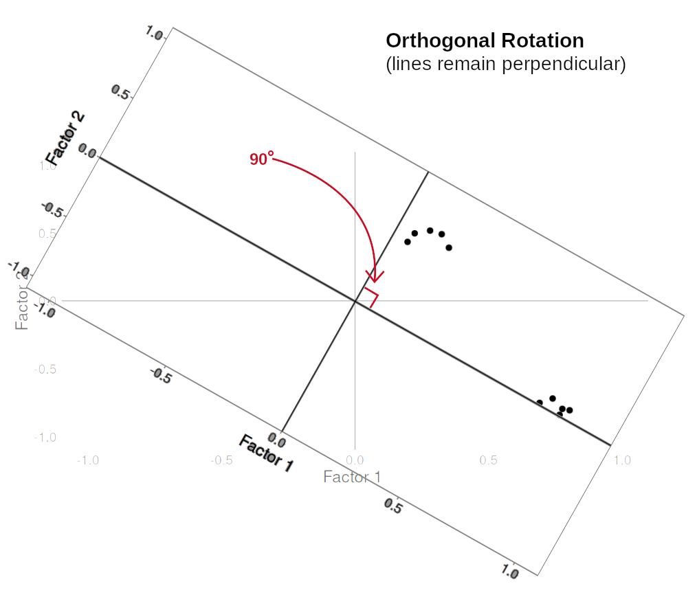
Figure 4: Orthogonal rotation
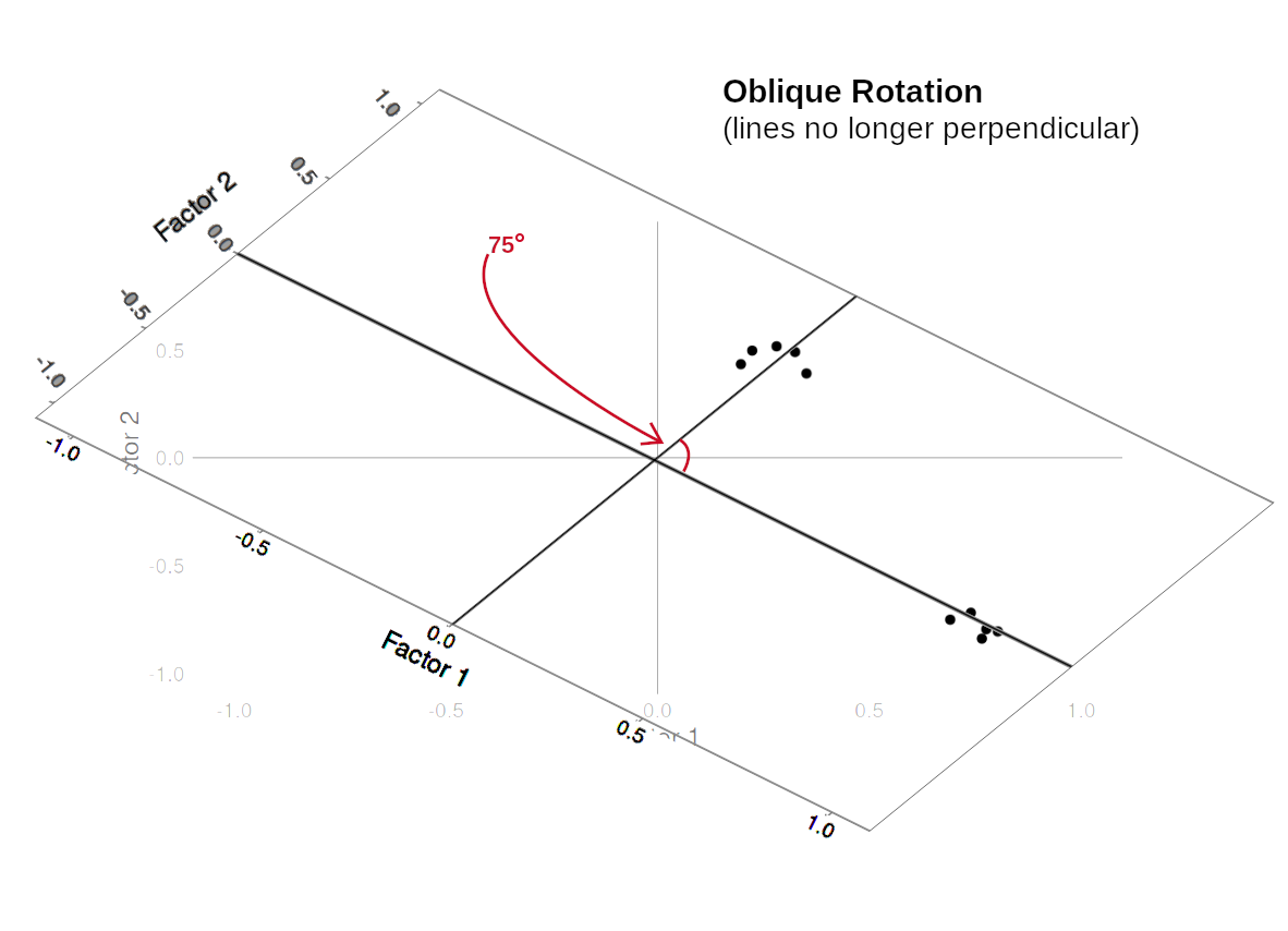
Figure 5: Oblique rotation
In our path diagram of the model (Figure 6), all the factor loadings remain present, but some of them become negligible. We can also introduce the possible correlation between our factors, as indicated by the curved arrow between \(F_1\) and \(F_2\).
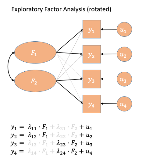
Figure 6: Path diagrams for EFA with rotation
Factor Extraction
PCA (using eigendecomposition) is itself a method of extracting the different dimensions from our data. However, there are lots more available for factor analysis.
You can find a lot of discussion about different methods both in the help documentation for the fa() function from the psych package:
Factoring method fm=“minres” will do a minimum residual as will fm=“uls”. Both of these use a first derivative. fm=“ols” differs very slightly from “minres” in that it minimizes the entire residual matrix using an OLS procedure but uses the empirical first derivative. This will be slower. fm=“wls” will do a weighted least squares (WLS) solution, fm=“gls” does a generalized weighted least squares (GLS), fm=“pa” will do the principal factor solution, fm=“ml” will do a maximum likelihood factor analysis. fm=“minchi” will minimize the sample size weighted chi square when treating pairwise correlations with different number of subjects per pair. fm =“minrank” will do a minimum rank factor analysis. “old.min” will do minimal residual the way it was done prior to April, 2017 (see discussion below). fm=“alpha” will do alpha factor analysis as described in Kaiser and Coffey (1965)
And there are lots of discussions both in papers and on forums.
As you can see, this is a complicated issue, but when you have a large sample size, a large number of variables, for which you have similar communalities, then the extraction methods tend to agree. For now, don’t fret too much about the factor extraction method.2
Use the function fa() from the psych package to conduct and EFA to extract 2 factors (this is what we suggest based on the various tests above, but you might feel differently - the ideal number of factors is subjective!). Use a suitable rotation and extraction method (fm).
conduct_efa <- fa(data, nfactors = ?, rotate = ?, fm = ?)
Inspect
DETAILS
If we think about a factor analysis being a set of regressions (convention in factor analysis is to use \( {\lambda_{,}} \) instead of \(\beta\)), then we can think of a given item being the manifestation of some latent factors, plus a bit of randomness:
\[\begin{aligned} \text{Item}_{1} &= {\lambda_{1,1}} \cdot \text{Factor}_{1} + {\lambda_{2,1}} \cdot \text{Factor}_{2} + u_{1} \\ \text{Item}_{2} &= {\lambda_{1,2}} \cdot \text{Factor}_{1} + {\lambda_{2,2}} \cdot \text{Factor}_{2} + u_{2} \\ &\vdots \\ \text{Item}_{16} &= {\lambda_{1,16}} \cdot \text{Factor}_{1} + {\lambda_{2,16}} \cdot \text{Factor}_{2} + u_{16} \end{aligned}\]Loadings
As you can see from the above, the 16 different items all stem from the same two factors (\( \text{Factor}_{1} , \text{Factor}_{2} \)), plus some item-specific errors (\(u_{1}, \dots, u_{16}\)). The \( {\lambda_{,}} \) terms are called factor loadings, or “loadings” in short
Communality is sum of the squared factor loadings for each item.
Intuitively, for each row, the two \( {\lambda_{,}} \)s tell us how much each item depends on the two factors shared by the 16 items. The sum of the squared loadings tells us how much of one item’s information is due to the shared factors.
The communality is a bit like the \(R^2\) (the proportion of variance of an item that is explained by the factor structure).
The uniqueness of each item is simply \(1 - \text{communality}\).
This is the leftover bit; the variance in each item that is left unexplained by the latent factors.
Side note: this is what sets Factor Analysis apart from PCA, which is the linear combination of total variance (including error) in all our items. FA allows some of the variance to be shared by the underlying factors, and considers the remainder to be unique to the individual items (or, in another, error in how each item measures the construct).
The complexity of an item corresponds to how well an item reflects a single underlying construct. Specifically, it is \({(\sum \lambda_i^2)^2}/{\sum \lambda_i^4}\), where \(\lambda_i\) is the loading on to the \(i^{th}\) factor. It will be equal to 1 for an item which loads only on one factor, and 2 if it loads evenly on to two factors, and so on.
In R, we will often see these estimats under specific columns:
- h2 = item communality
- u = item uniqueness
- com = item complexity
Inspect the loadings (conduct_efa$loadings) and give the factors you extracted labels based on the patterns of loadings.
Look back to the description of the items, and suggest a name for your factors
How correlated are your factors?
We can inspect the factor correlations (if we used an oblique rotation) using:
conduct_efa$Phi
Write-up
Drawing on your previous answers and conducting any additional analyses you believe would be necessary to identify an optimal factor structure for the 10 conduct problems, write a brief text that summarises your method and the results from your chosen optimal model.
PCA EFA Comparison exercise
Using the same data, conduct a PCA using the principal() function.
What differences do you notice compared to your EFA?
Do you think a PCA or an EFA is more appropriate in this particular case?
Even if we cut open someone’s brain, it’s unclear what we would be looking for in order to ‘measure’ it. It is unclear whether anxiety even exists as a physical thing, or rather if it is simply the overarching concept we apply to a set of behaviours and feelings↩︎
(It’s a bit like the optimiser issue in the multi-level model block)↩︎
You should provide the table of factor loadings. It is conventional to omit factor loadings \(<|0.3|\); however, be sure to ensure that you mention this in a table note.↩︎