Longitudinal (non-linear)
Preliminaries
Create a new R Script or RMarkdown document (whichever you prefer working with) and give it a title for this week.
Some extra background reading
We have already seen in the last couple of weeks that we can use MLM to study something ‘over the course of X’. In the novel word learning experiment from last week’s lab, we investigated the change in the probability of answering correctly over the course of the experimental blocks.
We’ve talked about how “longitudinal” is the term commonly used to refer to any data in which repeated measurements are taken over a continuous domain. This opens up the potential for observations to be unevenly spaced, or missing at certain points. It also, as will be the focus of this week, opens the door to thinking about how many effects of interest are likely to display non-linear patterns. These exercises focus on including higher-order polynomials in the multi-level model to capture non-linearity.
Linear vs Non-Linear
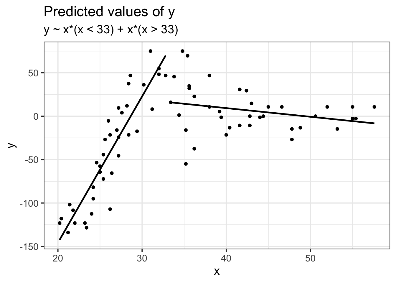
Suppose we had collected the data in Figure 1, and we wanted to fit a model to predict \(y\) based on the values of \(x\).
Let’s use our old friend linear regression, \(y = \beta_0 + \beta_1(x) + \varepsilon\).
We’ll get out some estimated coefficients, some standard errors, and some p-values:
- The intercept:
\(\beta_0\) = -110.28, SE = 19.54, p < .001
- The estimated coefficient of x:
\(\beta_1\) = 2.71, SE = 0.55, p < .001
Job done? Clearly not - we need only overlay model upon raw data (Figure 2) to see we are missing some key parts of the pattern.
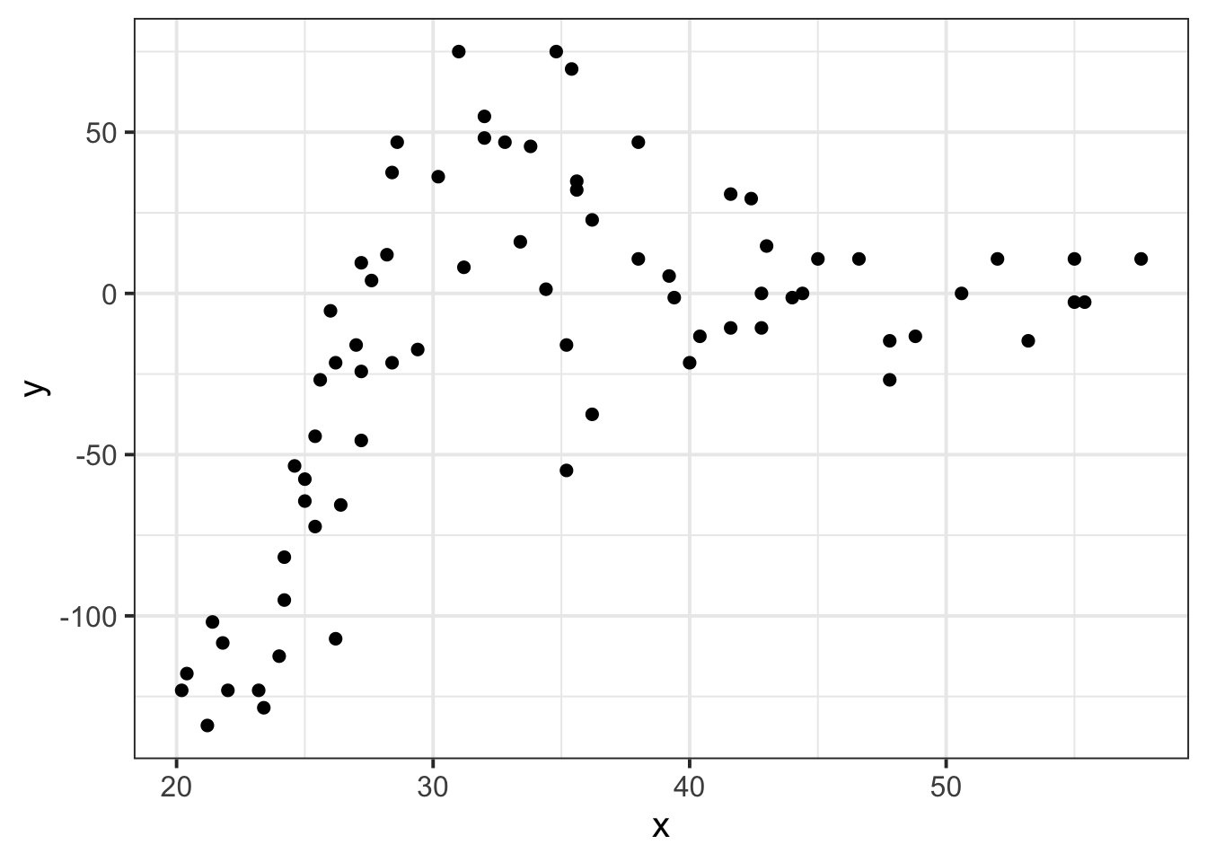
Figure 1: A clearly non-linear pattern
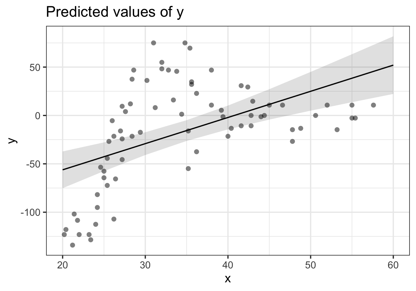
Figure 2: Uh-oh…
Thoughts about Model + Error
All our work here is in aim of making models of the world.
- Models are just models. They are simplifications, and so they don’t perfectly fit to the observed world (indeed, how well a model fits to the world is often our metric for comparing models).
- \(y - \widehat{y}\). Our observed data minus our model predicted values (i.e. in linear regression our “residuals”) reflect everything that we don’t account for in our model
- In an ideal world, our model accounts for all the systematic relationships, and what is left over (our residuals) is just randomness. If our model is mis-specified, or misses out something systematic, then our residuals will reflect this.
- We check for this by examining how much like randomness the residuals appear to be (zero mean, normally distributed, constant variance, i.i.d (“independent and identically distributed”) - i.e., what gets referred to as the “assumptions”).
- We will never know whether our residuals contain only randomness, because we can never observe everything.
Let’s just do a quick plot(model) for some diagnostic plots of my linear model:
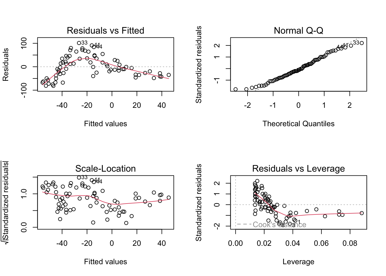
Does it look like the residuals are independently distributed? Not really. We need to find some way of incorporating the non-linear relationship between y and x into our model.
What is a polynomial?
Polynomials are mathematical expressions which involve a sum of powers. For instance:
- \(y = 4 + x + x^2\) is a second-order polynomial as the highest power of \(x\) that appears is \(x^2\)
- \(y = 9x + 2x^2 + 4x^3\) is a third-order polynomial as the highest power of \(x\) that appears is \(x^3\)
- \(y = x^6\) is a sixth-order polynomial as the highest power of \(x\) that appears is \(x^6\)
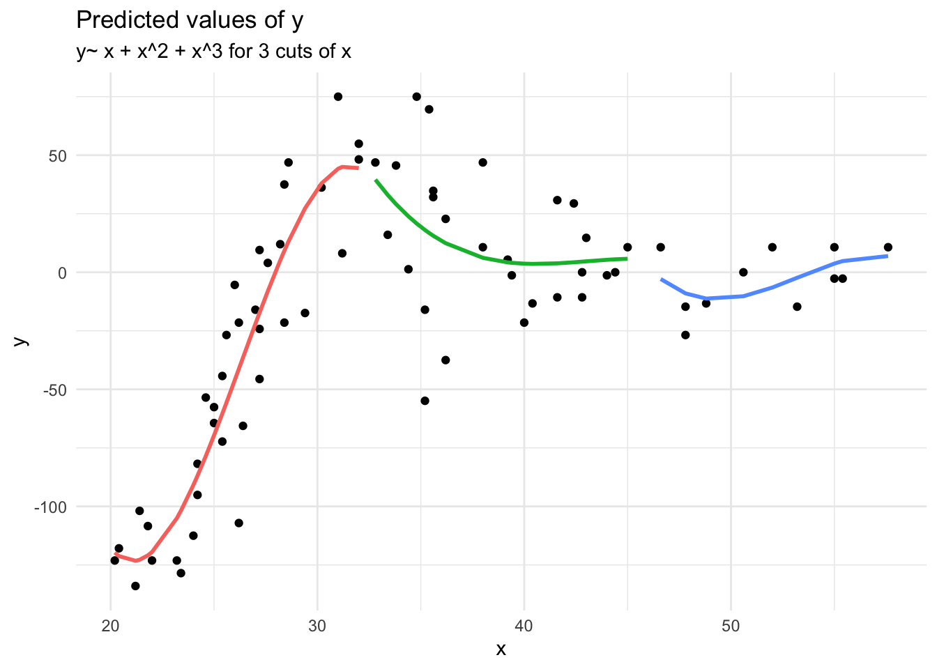
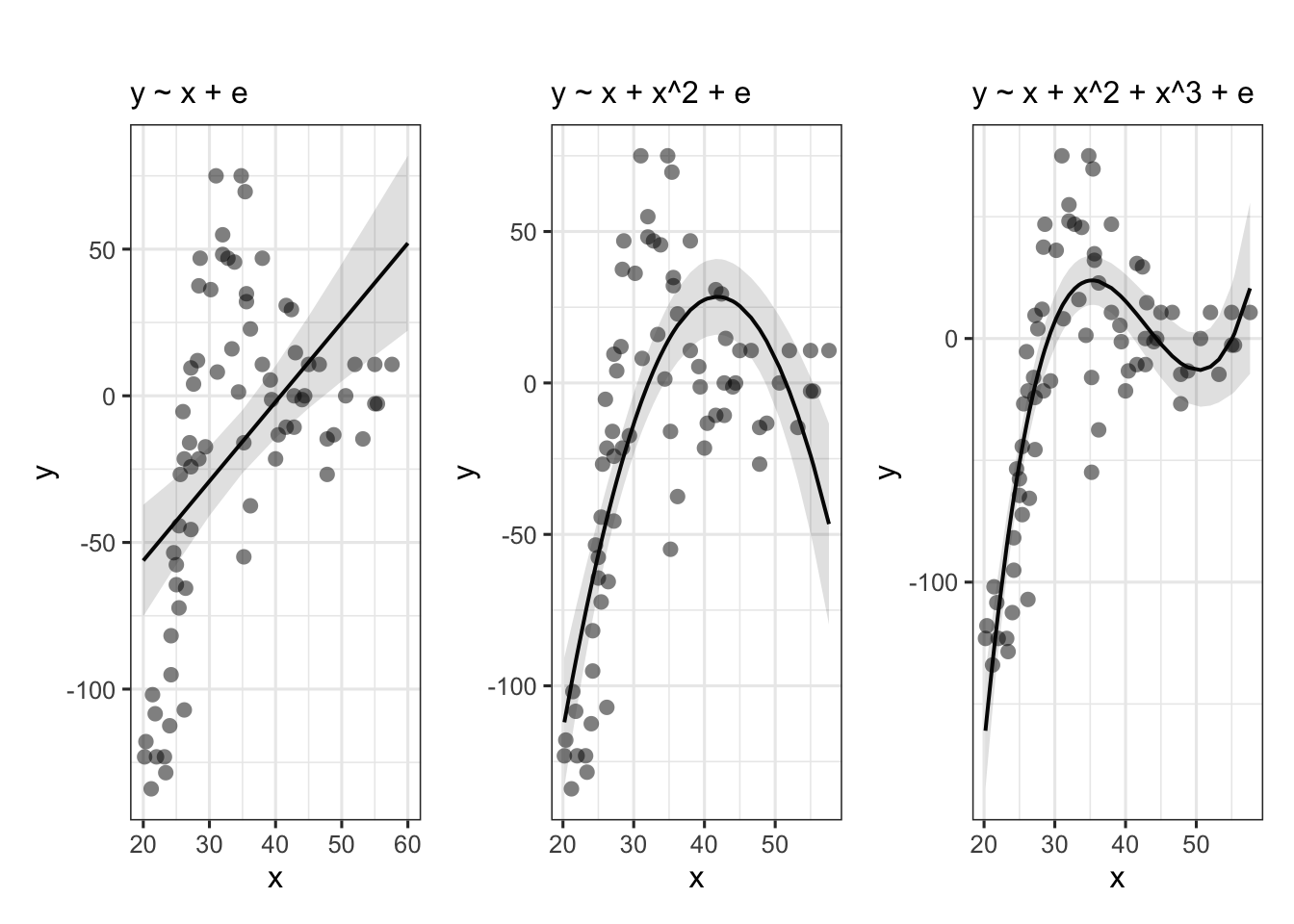
For our purposes, extending our model to include higher-order terms can fit non-linear relationships between two variables. For instance, fitting models with linear and quadratic terms (\(y_i\) = \(\beta_0 + \beta_1 x_{i} \ + \beta_2 x^2_i + \varepsilon_i\)) and extending these to cubic (\(y_i\) = \(\beta_0 + \beta_1 x_{i} \ + \beta_2 x^2_i + \beta_3 x^3_i + \varepsilon_i\)) (or beyond), may aid in modelling nonlinear patterns.
What are we interested in here?
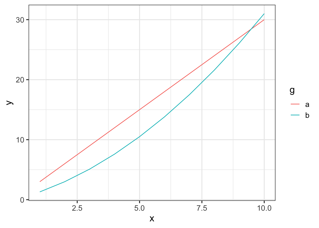
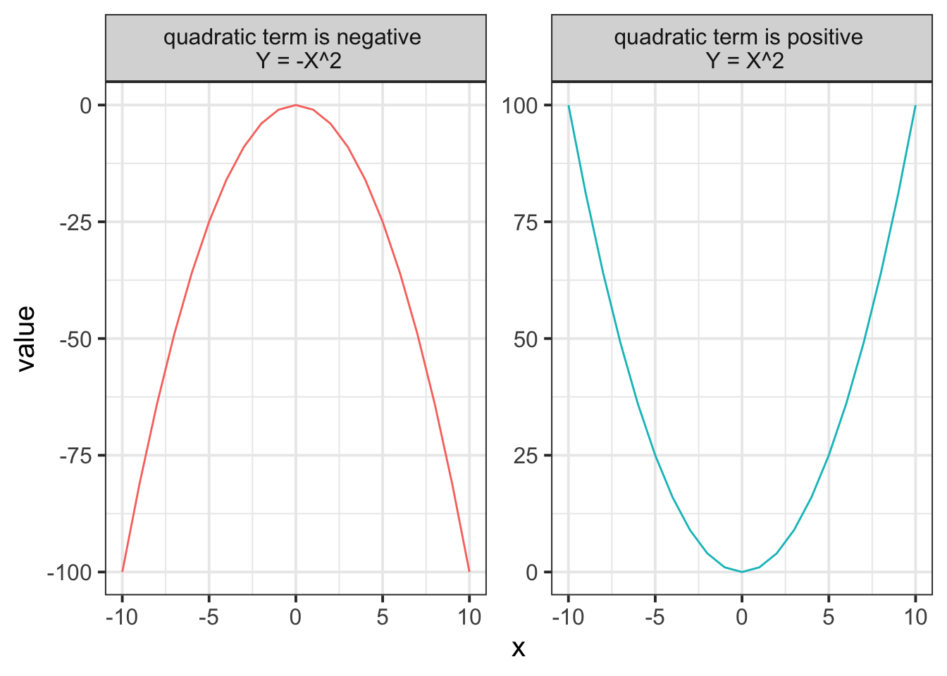
As the order of polynomials increases, we tend to be less interested in these terms in our model. Linear change is the easiest to think about: are things going up over the course of \(x\), or down? (or neither?). Quadratic change is the next most interesting, and it may help to think of this as the “rate of change”. For instance, in the plot below, it is the quadratic term which differs between the two groups trajectories.
Raw Polynomials
There are two types of polynomial we can construct. “Raw” (or “Natural”) polynomials are the straightforward ones you might be expecting the table to the right to be filled with.
These are simply the original values of the x variable to the power of 2, 3 and so on.
We can quickly get these in R using the poly() function, with raw = TRUE.
If you want to create “raw” polynomials, make sure to specify raw = TRUE or you will not get what you want because the default behaviour is raw = FALSE.
| x | x^2 | x^3 |
|---|---|---|
| 1 | ? | ? |
| 2 | ? | ? |
| 3 | ? | ? |
| 4 | ? | ? |
| 5 | ? | ? |
| … | … | … |
poly(1:10, degree = 3, raw=TRUE)## 1 2 3
## [1,] 1 1 1
## [2,] 2 4 8
## [3,] 3 9 27
## [4,] 4 16 64
## [5,] 5 25 125
## [6,] 6 36 216
## [7,] 7 49 343
## [8,] 8 64 512
## [9,] 9 81 729
## [10,] 10 100 1000
## attr(,"degree")
## [1] 1 2 3
## attr(,"class")
## [1] "poly" "matrix"Raw polynomials are correlated
With raw (or “natural”) polynomials, the terms poly1, poly2 and poly3 are correlated.
Think think about why this might be - by definition, as \(x^1\) increases, so will \(x^2\), and so will \(x^3\) and so on.
We can visualise them:
matplot(poly(1:10, 3, raw=T), type="l")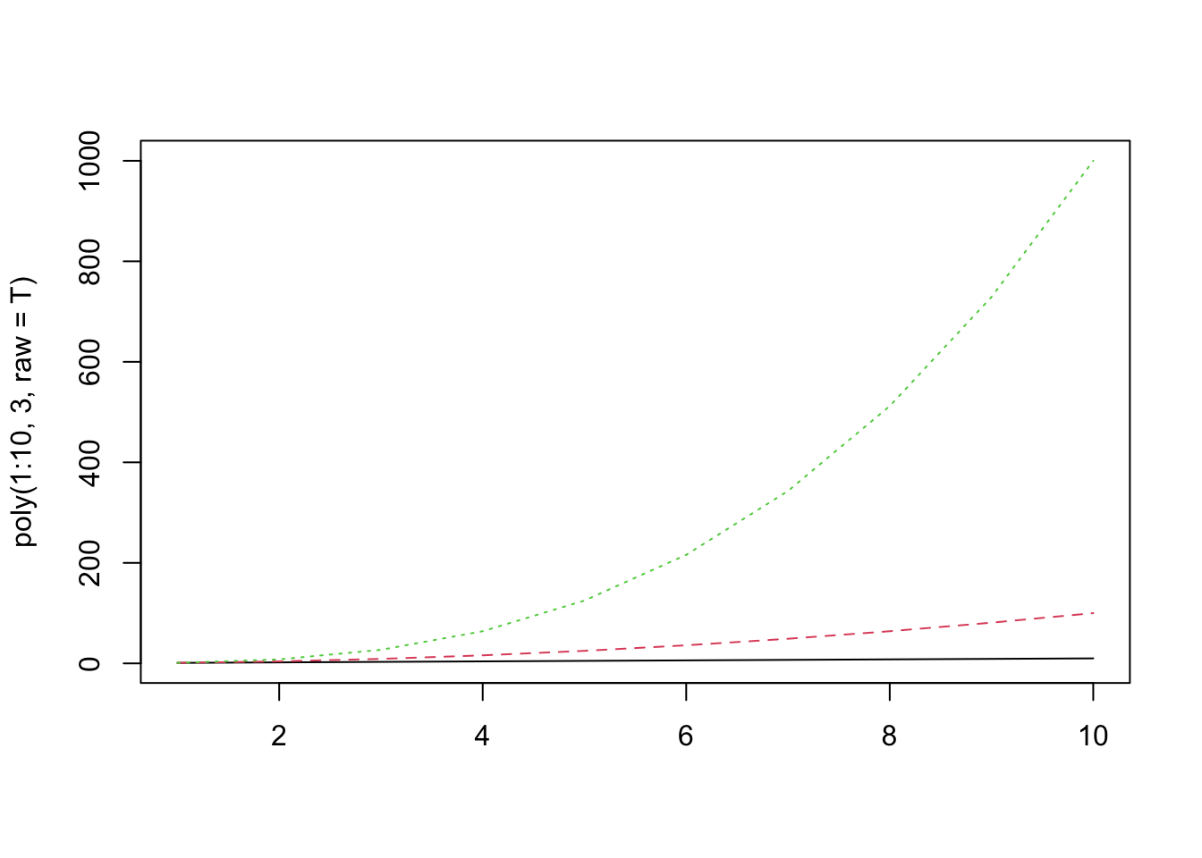 And measure the correlation coefficients:
cor(poly(1:10, 3, raw=T)) %>% round(2)## 1 2 3
## 1 1.00 0.97 0.93
## 2 0.97 1.00 0.99
## 3 0.93 0.99 1.00Well, this multicollinearity can lead to estimation problems, and means that our parameter estimates may change considerably depending upon what terms we include in our model, and it becomes more difficult to determine which ones are important, and what the effect sizes are.
Table 1 below shows the coefficients for models fitted to a randomly generated dataset, with
poly1, poly1+poly2, and poly1+poly2+poly3 as predictors (where poly1-poly3 are natural polynomials). Notice that they change with the addition of each term.
| term | y~poly1 | y~poly1+poly2 | y~poly1+poly2+poly3 |
|---|---|---|---|
| (Intercept) | 639.37 | -199.68 | -0.12 |
| poly1 | -144.01 | 275.52 | 98.52 |
| poly2 |
|
-38.14 | 0.24 |
| poly3 |
|
|
-2.33 |
Orthogonal Polynomials
“Orthogonal” polynomials are uncorrelated (hence the name). We can get these for \(x = 1,2,...,9,10\) using the following code:
poly(1:10, degree = 3, raw = FALSE)## 1 2 3
## [1,] -0.49543369 0.52223297 -0.4534252
## [2,] -0.38533732 0.17407766 0.1511417
## [3,] -0.27524094 -0.08703883 0.3778543
## [4,] -0.16514456 -0.26111648 0.3346710
## [5,] -0.05504819 -0.34815531 0.1295501
## [6,] 0.05504819 -0.34815531 -0.1295501
## [7,] 0.16514456 -0.26111648 -0.3346710
## [8,] 0.27524094 -0.08703883 -0.3778543
## [9,] 0.38533732 0.17407766 -0.1511417
## [10,] 0.49543369 0.52223297 0.4534252
## attr(,"coefs")
## attr(,"coefs")$alpha
## [1] 5.5 5.5 5.5
##
## attr(,"coefs")$norm2
## [1] 1.0 10.0 82.5 528.0 3088.8
##
## attr(,"degree")
## [1] 1 2 3
## attr(,"class")
## [1] "poly" "matrix"Notice that the first order term has been scaled, so instead of the values 1 to 10, we have values ranging from -0.5 to +0.5, centered on 0.
colMeans(poly(1:10, degree = 3, raw = FALSE)) %>%
    round(2)
## 1 2 3
## 0 0 0As you can see from the output above, which computes the mean of each column, each predictor has mean 0, so they are mean-centred. This is a key fact and will affect the interpretation of our predictors later on.
Think about what this means for \(x^2\). It will be uncorrelated with \(x\) (because \(-0.5^2 = 0.5^2\))!
matplot(poly(1:10, 3, raw=F), type="l")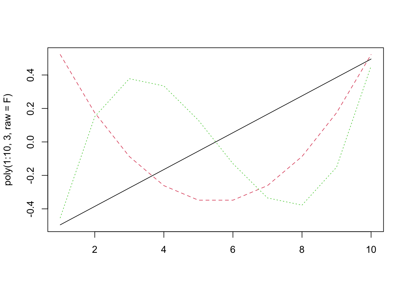 The correlations are zero!
cor(poly(1:10, 3, raw=F)) %>% round(2)## 1 2 3
## 1 1 0 0
## 2 0 1 0
## 3 0 0 1y~poly1, y~poly1+poly2, and y~poly1+poly2+poly3 as predictors (where poly1-poly3 are now orthogonal polynomials), and see that estimated coefficients do not change between models:
| term | y~poly1 | y~poly1+poly2 | y~poly1+poly2+poly3 |
|---|---|---|---|
| (Intercept) | -152.66 | -152.66 | -152.66 |
| poly1 | -1307.99 | -1307.99 | -1307.99 |
| poly2 |
|
-876.36 | -876.36 |
| poly3 |
|
|
-129.26 |
Remember what zero is!
With orthogonal polynomials, you need to be careful about interpreting coefficients. For raw polynomials the intercept remains the y-intercept (i.e., where the line hits the y-axis). The higher order terms can then be thought of from that starting point - e.g., “where \(x\) is 2, \(\widehat{y}\) is \(\beta_0 + \beta_1 \cdot 2 + \beta_2 \cdot 2^2 + \beta_3 \cdot 2^3 ...\)”.
For orthogonal polynomials, the interpretation becomes more tricky. The intercept is the overall average of y, the linear predictor is the linear change pivoting around the mean of \(x\) (rather than \(x = 0\)), the quadratic term corresponds to the steepness of the quadratic curvature (“how curvy is it?”), the cubic term to the steepness at the inflection points (“how wiggly is it?”), and so on.
Some useful code from Dan
It’s possible to use poly() internally in fitting our linear model, if we want:
lm(y ~ poly(x, 3, raw = T), data = df)
Unfortunately, the coefficients will end up having long messy names poly(x, 3, raw = T)[1], poly(x, 3, raw = T)[2] etc.
It is probably nicer if we add the polynomials to our data itself. As it happens, Dan has provided a nice little function which attaches these as columns to our data, naming them poly1, poly2, etc.
# import Dan's code and make it available in our own R session
# you must do this in every script you want to use this function
source("https://uoepsy.github.io/msmr/functions/code_poly.R")

mydata <- code_poly(df = mydata, predictor = 'time', poly.order = 3,
                    orthogonal = FALSE, draw.poly = FALSE)
head(mydata)
## # A tibble: 6 × 6
## time y time.Index poly1 poly2 poly3
## <int> <dbl> <dbl> <dbl> <dbl> <dbl>
## 1 1 96.8 1 1 1 1
## 2 2 179. 2 2 4 8
## 3 3 234. 3 3 9 27
## 4 4 248. 4 4 16 64
## 5 5 209. 5 5 25 125
## 6 6 97.2 6 6 36 216Both will produce the same model output (but Dan’s method produces these nice neat names for the coefficients!), and we can just put the terms into our model directly as lm(y ~ poly1 + poly2 + poly3, data = mydata).
Exercises: Cognitive performance
STOP AND THINK: Are you using R effectively?
There are lots of different ways to organise your file system/your life in R. You might be creating a new project each week, or a new folder, or just a new .Rmd. There’s no best way to organise this - it is personal preference.
However, one thing which is common across most approaches is that having a lot of irrelevant stuff in your environment (top right pane) can get confusing and messy.
We encourage you now to clear your environment for this week, and then load in the data.
If you are worried that you are going to lose some of the objects in your environment, then this may be a sign that you are not using R to its full potential. The idea is that we can recreate all of our analyses by just running the relevant code in our script!
Alongside lme4 and tidyverse and possibly broom.mixed, we’re going to be using some of Dan’s useful functions for getting p-values and coding polynomials.
The source() function basically takes in R code and evaluates it. You can download an R script with Dan’s code here.
But you can also source this script directly from the URL, which runs the R code and creates the functions in your environment. Typically, we want these at the top of our document, because it’s similar to loading a package:
library(tidyverse)
library(lme4)
library(broom.mixed)
source("https://uoepsy.github.io/msmr/functions/code_poly.R")
Az.rda Data
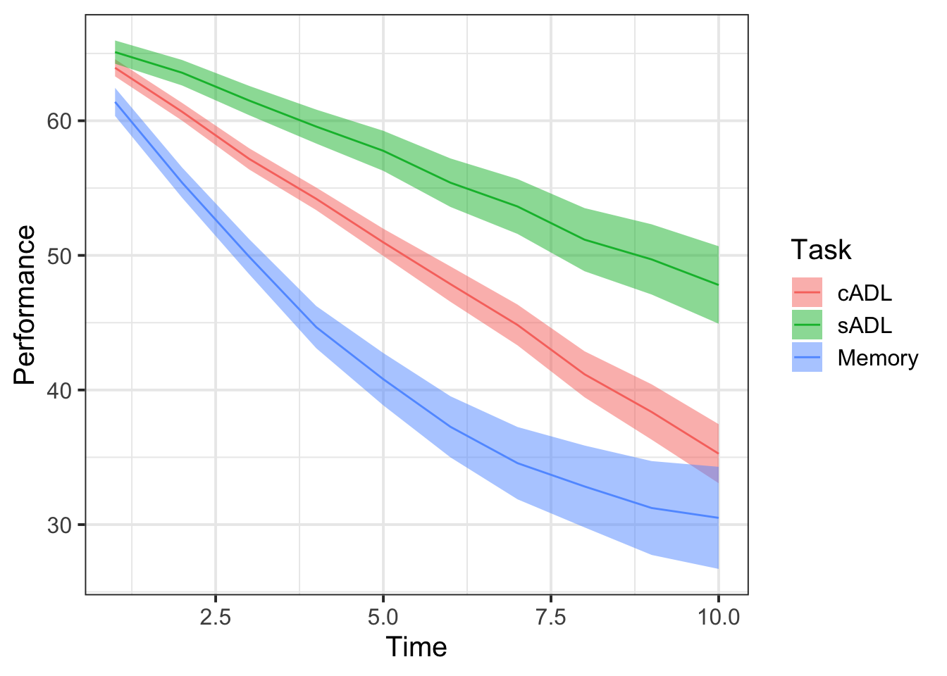
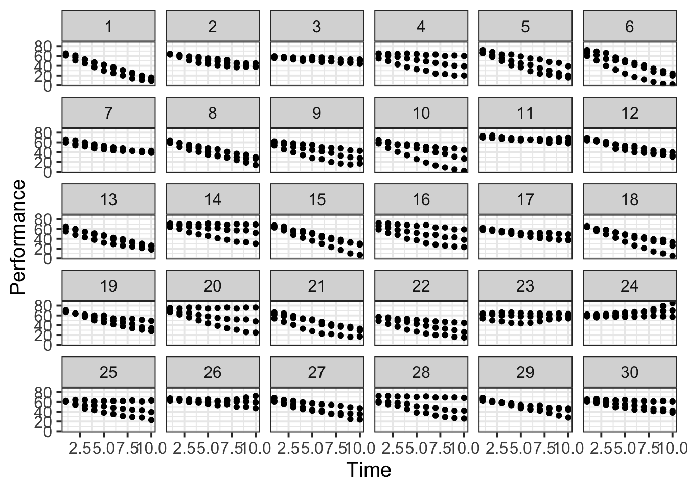
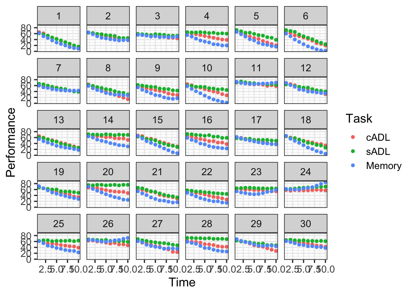
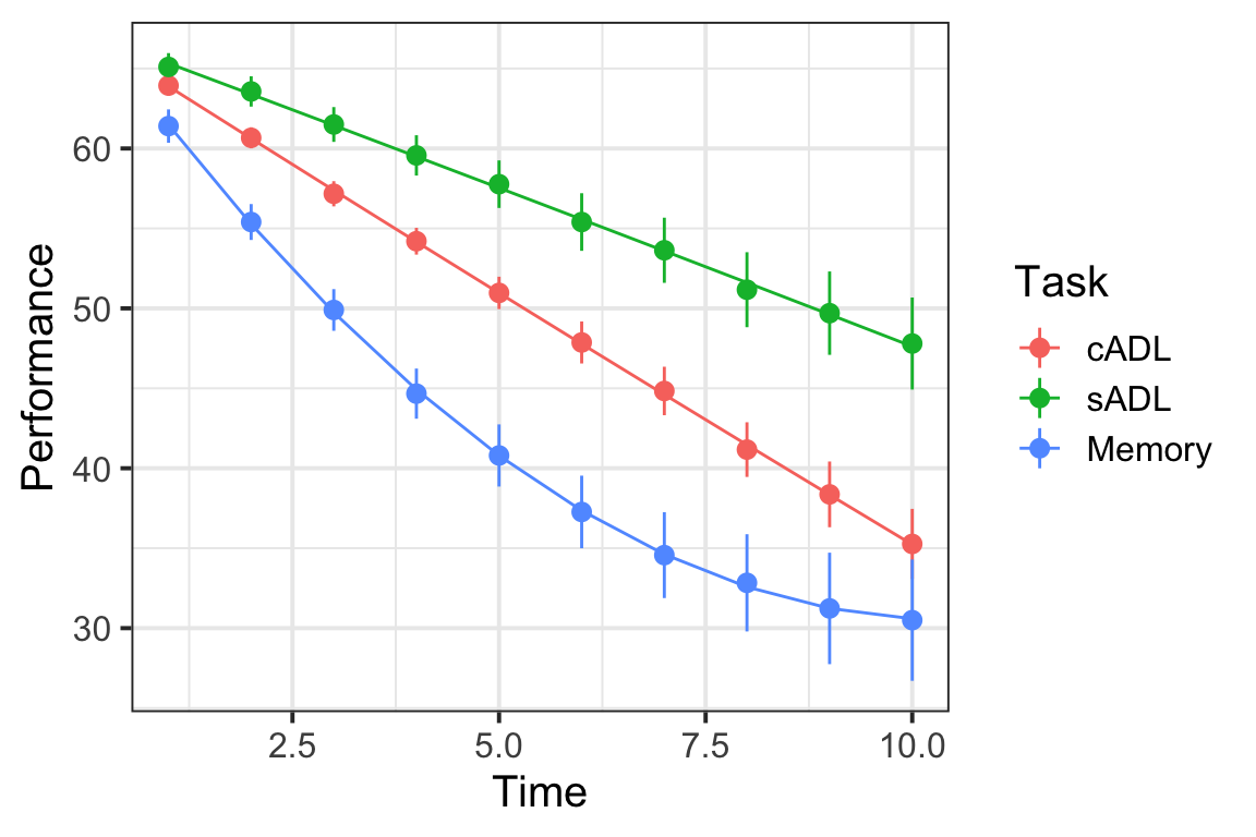
30 Participants with probably Alzheimer’s Disease completed 3 tasks over 10 time points: A memory task, and two scales investigating ability to undertake complex activities of daily living (cADL) and simple activities of daily living (sADL). Performance on all of tasks was calculated as a percentage of total possible score, thereby ranging from 0 to 100.
The data is available at https://uoepsy.github.io/data/Az.rda.
| variable | description |
|---|---|
| Subject | Unique Subject Identifier |
| Time | Time point of the study (1 to 10) |
| Task | Task type (Memory, cADL, sADL) |
| Performance | Score on test |
Load in the data and examine it.
No modelling just yet.
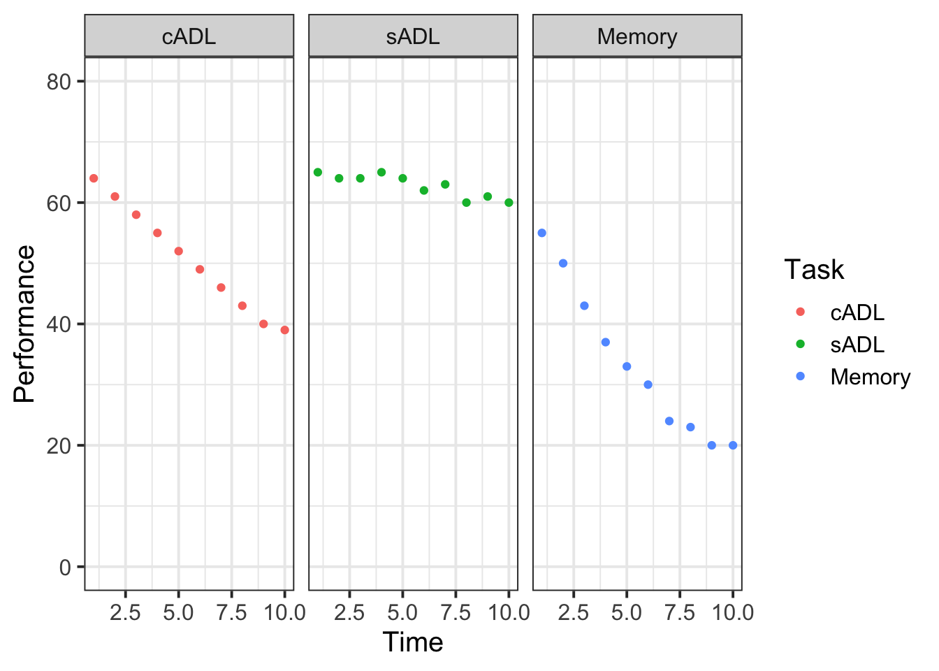
Plot the performance over time for each type of task.
Try using stat_summary so that you are plotting the means (and standard errors) of each task, rather than every single data point. Why? Because this way you can get a shape of the overall trajectories of performance over time in each task.
Why do you think raw/natural polynomials might be more useful than orthogonal polynomials for these data?
Okay! Let’s do some modeling!
First steps:
- Add 1st and 2nd order raw polynomials to the data using the
code_poly()function. - Create a “baseline model”, in which performance varies over time (with both linear and quadratic change), but no differences in Task are estimated.
We need to think about our random effect structure. We’ll talk you through this bit because it’s getting a bit more complicated now.
Hopefully, you fitted a model like this (or thereabouts)
m.base <- lmer(Performance ~ (poly1 + poly2) +
(1 + poly1 + poly2 | Subject/Task),
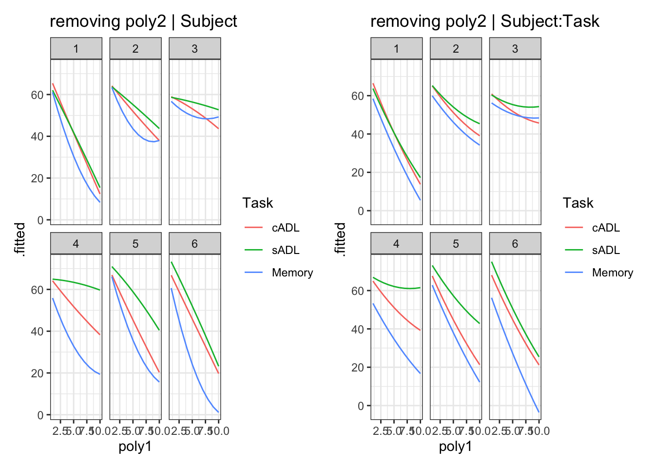
data=Az, REML=F, control=lmerControl(optimizer="bobyqa"))Remember what we learned last week about “singular fits”? It looks like this model might be a too complex for the data to sustain.
What random effect term might we consider removing? (there isn’t necessarily a “right” answer here - many may be defensible, but your decision should be based on multiple considerations/evidence).
Let’s start adding in our effects of interest.
- Create a new model with a fixed effect of Task
- Create a new model in which performance varies linearly over time between Task type.
- Create a new model in which linear and quadratic performance over time varies between Task type.
- Run model comparisons.
We’d like to do some inferential tests of our coefficients values. We could consider computing some confidence intervals with confint(m.Az.full, method="boot"), but this may take quite a long time with such a complex model (if we bootstrap, we’re essentially fitting thousands of models!).
For now, let’s refit the full model and obtain p-values for our coefficients by using the Satterthwaite approximations for the denominator degrees of freedom.
The code below does this for us
By using lmerTest::lmer() we don’t have to load the package library(lmerTest), and so it is just this single model that’s get fitted this way.
m.full_satter <-
    lmerTest::lmer(Performance ~ (poly1 + poly2) * Task +
                       (1 + poly1 | Subject) + (1 + poly1 + poly2 | Subject:Task),
                   data=Az, REML=F, control=lmerControl(optimizer="bobyqa"))

tidy(m.full_satter) %>%
    filter(effect=="fixed")
## # A tibble: 9 × 8
## effect group term estimate std.error statistic df p.value
## <chr> <chr> <chr> <dbl> <dbl> <dbl> <dbl> <dbl>
## 1 fixed <NA> (Intercept) 67.2 0.927 72.5 51.1 3.66e-53
## 2 fixed <NA> poly1 -3.29 0.335 -9.80 48.9 3.94e-13
## 3 fixed <NA> poly2 0.00947 0.0124 0.762 90.0 4.48e- 1
## 4 fixed <NA> TasksADL 0.0950 0.812 0.117 60.0 9.07e- 1
## 5 fixed <NA> TaskMemory 1.24 0.812 1.53 60.0 1.32e- 1
## 6 fixed <NA> poly1:TasksADL 1.36 0.270 5.05 60.1 4.47e- 6
## 7 fixed <NA> poly1:TaskMemory -3.98 0.270 -14.7 60.1 1.32e-21
## 8 fixed <NA> poly2:TasksADL -0.0133 0.0176 -0.754 90.0 4.53e- 1
## 9 fixed <NA> poly2:TaskMemory 0.339 0.0176 19.3 90.0 1.07e-33
| term | estimate | std.error | statistic | df | p.value |
|---|---|---|---|---|---|
| (Intercept) | 67.16 | 0.93 | 72.48 | 51.06 | <.001 *** |
| poly1 | -3.29 | 0.34 | -9.80 | 48.95 | <.001 *** |
| poly2 | 0.01 | 0.01 | 0.76 | 90.00 | .448 |
| TasksADL | 0.10 | 0.81 | 0.12 | 60.05 | .907 |
| TaskMemory | 1.24 | 0.81 | 1.53 | 60.05 | .132 |
| poly1:TasksADL | 1.36 | 0.27 | 5.04 | 60.08 | <.001 *** |
| poly1:TaskMemory | -3.98 | 0.27 | -14.73 | 60.08 | <.001 *** |
| poly2:TasksADL | -0.01 | 0.02 | -0.75 | 90.00 | .453 |
| poly2:TaskMemory | 0.34 | 0.02 | 19.27 | 90.00 | <.001 *** |
- For the cADL Task, what is the estimated average performance where x = 0?
- For the sADL and Memory Tasks, is the estimated average where x = 0 different to the cADL Task?
- For the cADL Task, how does performance change for every increasing time point? (what is the estimated linear slope?)
- Note, the quadratic term
poly2is non-significant, so we’ll ignore it here
- Note, the quadratic term
- For the sADL Task, how is the change in performance over time different from the cADL Task?
- The answer to c) + the answer to d) will give you the estimated slope for the sADL Task.
- For the Memory task, how does performance change for every increasing time point? In other words, what is the slope for the Memory task and what effect does time have?
- This is more difficult. The quadratic term is significant.
- Recall the direction of the quadratic term (positive/negative) and how this relates to the visual curvature (see back in “What’s a polynomial?”).
Based on your answers above, can you sketch out (on paper) the model fit?
Then provide a written description.
To what extent do model comparisons (Question A6) and the parameter-specific p-values (Question A7) yield the same results?
Plot the model fitted values. This might be pretty similar to the plot you created in Question A2, and (hopefully) similar to the one you drew on paper for Question A8.
Two quotes
“all models are wrong. some are useful.” (George Box, 1976).
“…it does not seem helpful just to say that all models are wrong. The very word model implies simplification and idealization. The idea that complex physical, biological or sociological systems can be exactly described by a few formulae is patently absurd. The construction of idealized representations that capture important stable aspects of such systems is, however, a vital part of general scientific analysis and statistical models, especially substantive ones, do not seem essentially different from other kinds of model.”(Sir David Cox, 1995).