Writing-up
A sample question
We saw in the lecture a brief explanation of approaching the following sample question from a previous year’s coursework report:
Sample Question: Driving speeds, night vs. day
Does time of day and speed of driving predict the blood alcohol content over and above driver’s age? Fit appropriate model(s) to test this question, and report the results (you may add a figure or table if appropriate).
Drinkdriving Data
Two datasets can be loaded from the following url:
load(url("https://uoepsy.github.io/data/usmr_1920_assignment.RData"))The data provided contains information about the nature and circumstances of motorists stopped and breathalysed by the Police.
Data is collected every time that driver is stopped by the Police and breathalysed. Records indicate the speed at which the driver is travelling when they are stopped, and the blood alcohol content of the driver when measured via breathalyser. Information is also captured on the age and prior motoring offences of the driver, and whether the incident occurred at day or night. Police officers may have had reasons for stopping drivers other than presuming them to be intoxicated (for instance, someone who is stopped for speeding may subsequently be breathalysed if they are deemed to be acting unusually).
Each time a police officer stops a motorist, an incident ID is created. A separate database used primarily for administrative purposes includes records of which officer (recorded as initials) attends which incidents.
| Variable | Description |
|---|---|
| age | Age of driver (in years) |
| nighttime | Whether or not the incident occurred at night |
| prior_offence | Offence code for any prior motoring offences |
| speed | Speed when stopped by police (mph) |
| bac | Blood Alcohol Content (%) as measured by breathalyser |
| outcome | Outcome of stop ('fine','warning') |
| incident_id | ID of incident |
| officer | Officer attending (initials) |
Explore and clean the dataset (i.e., remove any impossible values etc).
Some info on the lecture slides this week will help with guidance on what to look for.
(for now, you can ignore things like the “prior_offence” variable if you want, as this is a tricky one to tidy up, and isn’t relevant for the sample question we are considering)
Take another look at our question:
Does time of day and speed of driving predict the blood alcohol content over and above driver’s age? Fit appropriate model(s) to test this question, and report the results (you may add a figure or table if appropriate).
Try to provide an answer (hint: we’re probably going to want to use lm() and/or anova()). Can you give extra context to your answer?
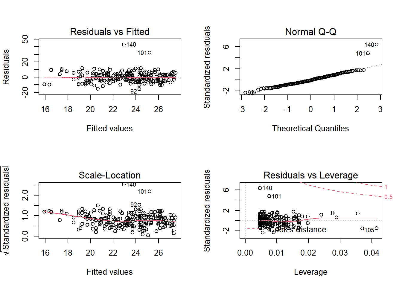
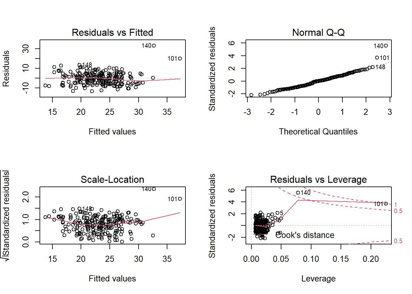 Which highlights a couple of points which seem to be extremely influential.
On further investigation, one of these observations seemed to be very fast (was the max speed observed) and both have recorded very high BAC values.
Which highlights a couple of points which seem to be extremely influential.
On further investigation, one of these observations seemed to be very fast (was the max speed observed) and both have recorded very high BAC values.
Writing-up Guide
Here, we’re going to walk through a high-level step-by-step guide of what to include in a write-up of a statistical analysis. We’re going to use an example analysis using one of the datasets we have worked with on a number of exercises in previous labs concerning personality traits, social comparison, and depression and anxiety.
The aim in writing should be that a reader is able to more or less replicate your analyses without referring to your R code. This requires detailing all of the steps you took in conducting the analysis.
The point of using RMarkdown is that you can pull your results directly from the code. If your analysis changes, so does your report!
You can find a .pdf of the take-everywhere write-up checklist here.
Research Question
Previous research has identified an association between an individual’s perception of their social rank and symptoms of depression, anxiety and stress. We are interested in the individual differences in this relationship.
Specifically:
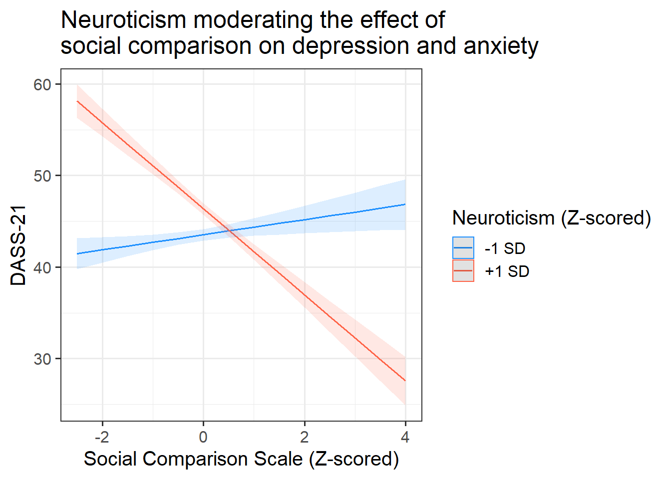
Research question: Controlling for other personality traits, does neuroticism moderate effects of social comparison on symptoms of depression, anxiety and stress?
1. Think
What do you know? What do you hope to learn? What did you learn during the exploratory analysis?
If you were reporting on your own study, then the first you would want to describe the study design, the data collection strategy, etc.
This is not necessary here, but we could always say something brief like:
Data was obtained from https://uoepsy.github.io/data/scs_study.csv: a dataset containing information on 656 participants
- How many observational units?
- Are there any observations that have been excluded based on pre-defined criteria? How/why, and how many?
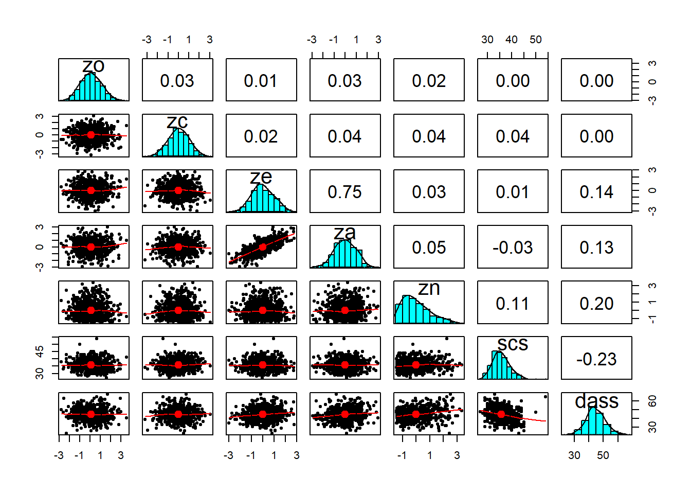
- Describe and visualise the variables of interest. How are they scored? have they been transformed at all?
- Describe and visualise relationships between variables. Report covariances/correlations.
- What type of statistical analysis do you use to answer the research question? (e.g., t-test, simple linear regression, multiple linear regression)
- Describe the model/analysis structure
- What is your outcome variable? What is its type?
- What are your predictors? What are their types?
- Any other specifics?
- Was there anything you had to do differently than planned during the analysis? Did the modelling highlight issues in your data?
- Did you have to do anything (e.g., transform any variables, exclude any observations) in order to meet assumptions?
2. Show
Show the mechanics and visualisations which will support your conclusions
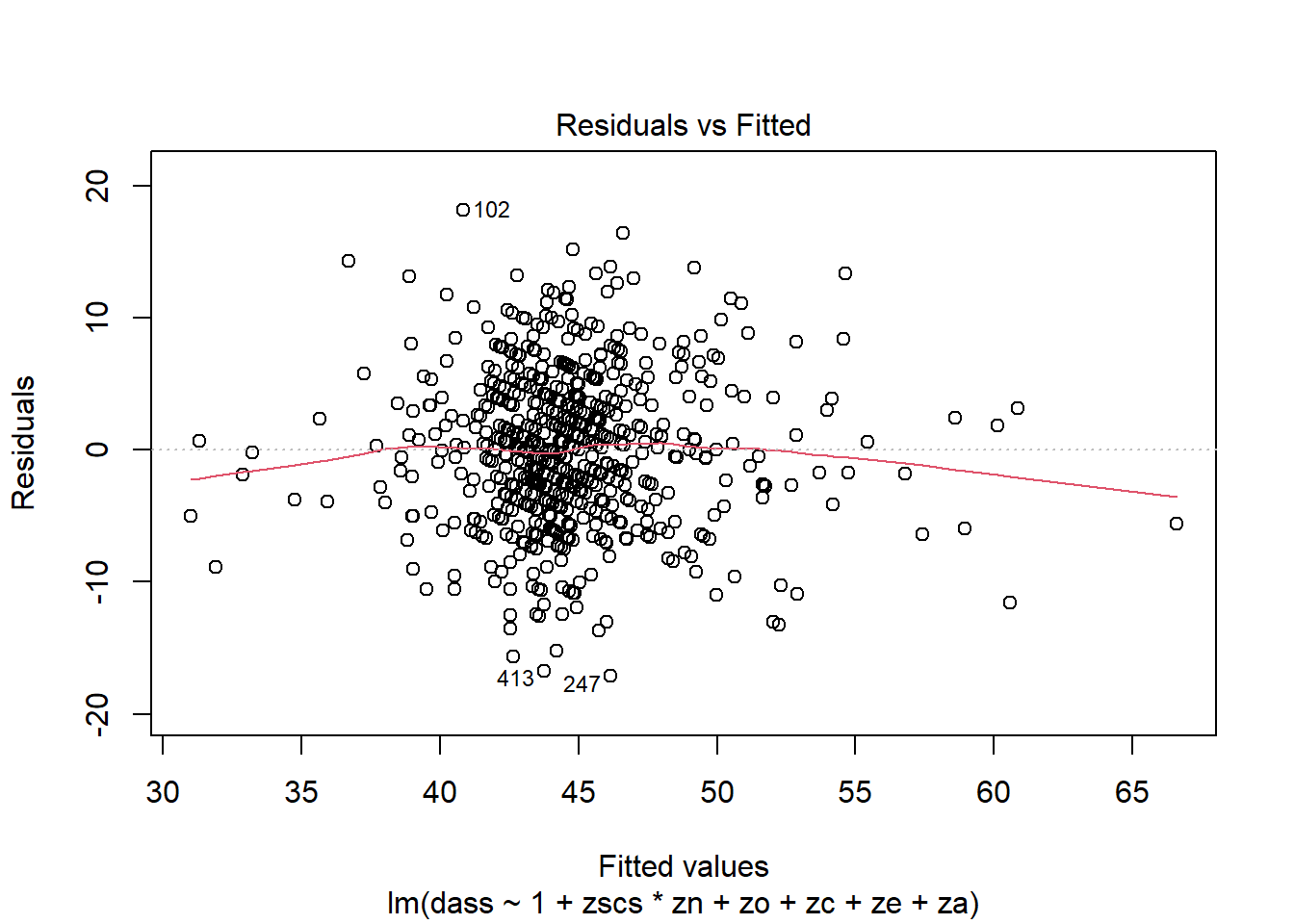
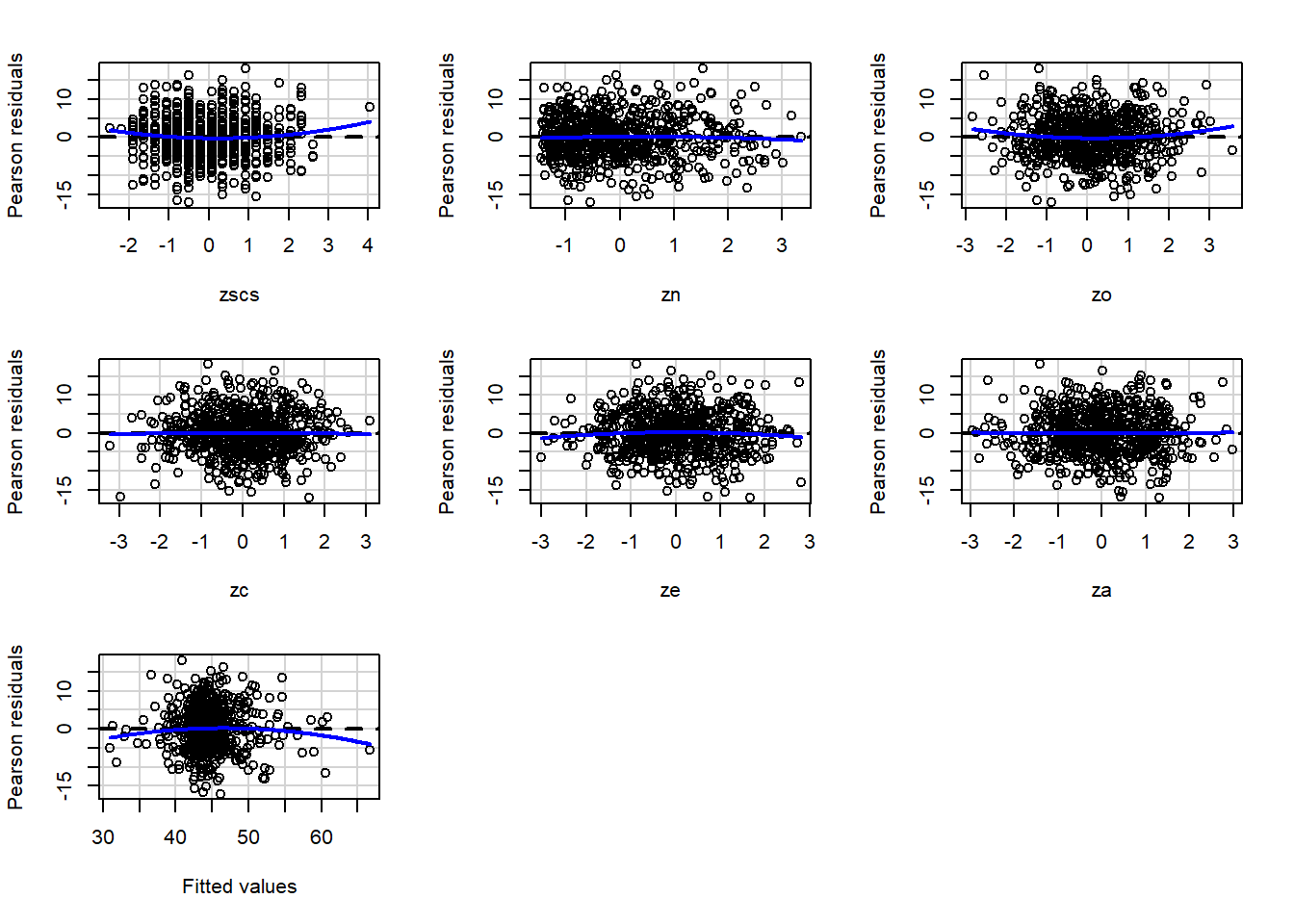
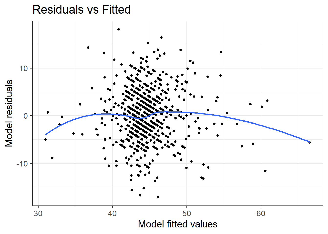
Present and describe the model or test which you deemed best to answer your question.
For the final model (the one you report results from), were all assumptions met? (Hopefully yes, or there is more work to do…). Include evidence (tests or plots).
- Provide a table of results if applicable (for regression tables, try
tab_model()from the sjPlot package).
- Provide plots if applicable.
3. Tell
Communicate your findings
- What do your results suggest about your research question?
- Make direct links from hypotheses to models (which bit is testing hypothesis)
- Be specific - which statistic did you use/what did the statistical test say? Comment on effect sizes.
- Make sure to include measurement units where applicable.
Tying it all together
All the component parts we have just written in the exercises above can be brought together to make a reasonable draft of a statistical report. There is a lot of variability in how to structure the reporting of statistical analyses, for instance you may be using the same model to test a selection of different hypotheses.
The answers contained within the solution boxes above are an example. While we hope it is useful for you when you are writing reports, dissertations etc, it should not be taken as an exemplary template for a report which would score 100%.
You can find an RMarkdown file which contains all these parts here, which may be useful to see how things such as formatting and using inline R code can be used.
Life Beyond USMR
Linear models and other things
Once you start using linear models, you might begin to think about how many other common statistical tests can be put into a linear model framework. Below are some very quick demonstrations of a couple of equivalences, but there are many more, and we encourage you to explore this further by a) playing around with R, and b) reading through some of the examples at https://lindeloev.github.io/tests-as-linear/.
Cheat Sheets
You can find many RStudio cheatsheets at https://rstudio.com/resources/cheatsheets/, but some of the more relevant ones to this course are listed below:
Thank you!
Lastly, we’d just like to say a big thank you for following all of our ramblings, for your attendance across the various sessions, and for all your excellent questions on Piazza. We hope that you feel that you have learned something this semester, and that it has been (at least in some ways) an enjoyable experience. Those of you who are planning on taking the Multivariate Stats (MSMR) course next semester are not free of us just yet - we’ll see you in January!
Josiah, Umberto & Emma

This workbook was written by Josiah King, Umberto Noe, and Martin Corley, and is licensed under a Creative Commons Attribution 4.0 International License.