More Linear Regression
Standardising Coefficients
Often it is useful to make distinctions in notation between the effects that we are interested in (the population parameter) and our best guess (the estimate). With regression coefficients this is the notation we tend to use in this course (there are many other conventions for notation):
| Population parameter | Fitted estimate |
|---|---|
| \(b\) | \(\hat b\) |
Remember the scale of your variables!
Recall one of our models from last week, explaining wellbeing by the combination of social interactions and outdoor time:
\[
\textrm{Wellbeing} = b_0 \ + \ b_1 (\textrm{Outdoor Time}) \ + \ b_2 (\textrm{Social Interactions}) \ +\ \epsilon
\]
We fitted this as so:
mwdata <- read_csv(file = "https://uoepsy.github.io/data/wellbeing.csv")
wbmodel2 <- lm(wellbeing ~ outdoor_time + social_int, data=mwdata)- Wellbeing: Warwick-Edinburgh Mental Wellbeing Scale (WEMWBS), a self-report measure of mental health and well-being. The scale is scored by summing responses to each item, with items answered on a 1 to 5 Likert scale. The minimum scale score is 14 and the maximum is 70.
- Social Interactions: Self report estimated number of social interactions per week (both online and in-person)
- Outdoor Time: Self report estimated number of hours per week spent outdoors
This influences our interpretation of the coefficients (the \(\hat b\)’s):
- \(\hat b_0\) = the estimated mean score on the WEMWBS for someone who has zero social interactions per week and zero hours of outdoor time per week.
- \(\hat b_1\) = for every increase in 1 hour of outdoor time per week, scores on the WEMWBS are estimated to change by \(\hat b_1\) points.
- \(\hat b_2\) = for every increase in 1 social interaction per week, scores on the WEMWBS are estimated to change by \(\hat b_2\) points.
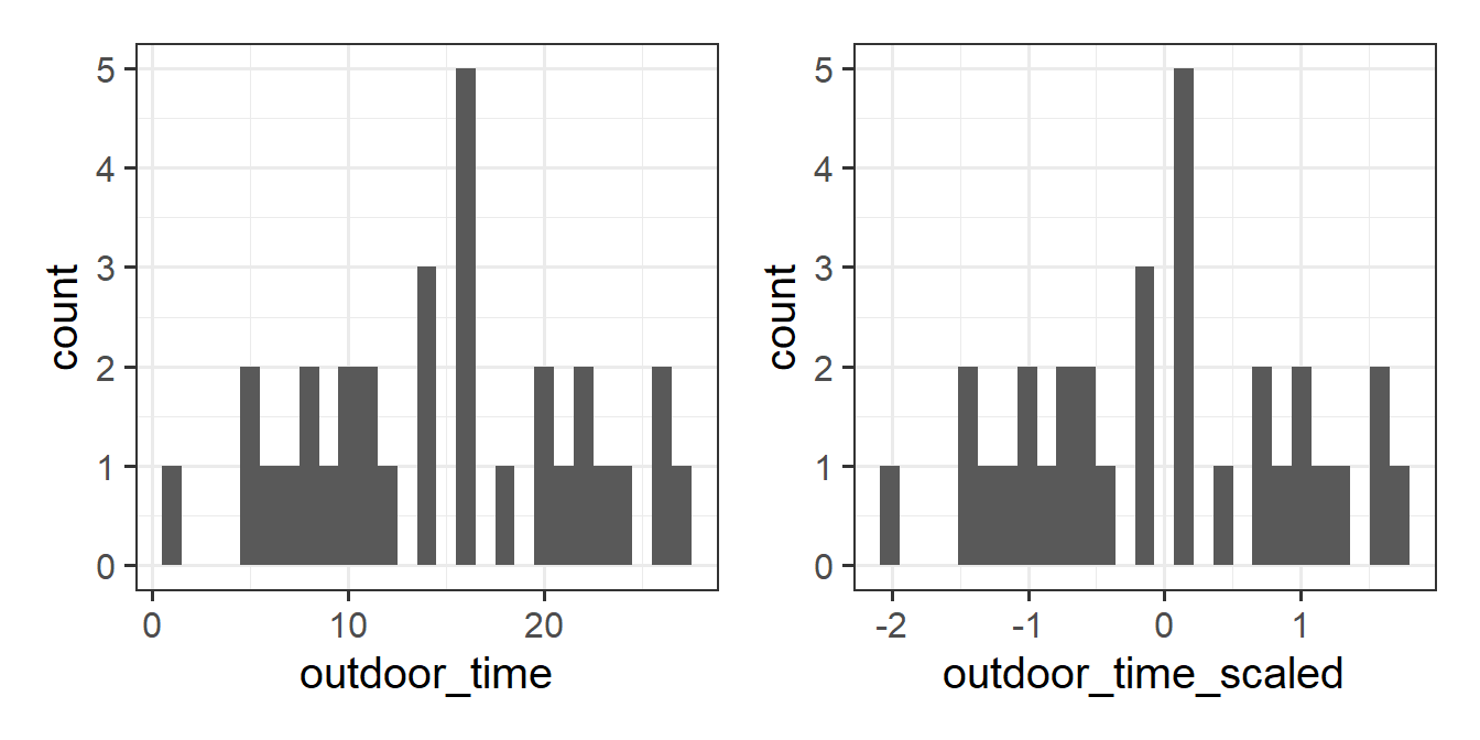
The code below creates a standardised the outdoor_time variable, transforming the values so that the mean of the new variable is 0, and the standard deviation is 1.
We can either use the scale() function to do this, or do it manually:
mwdata <- mwdata %>%
  mutate(
    outdoor_time_scaled = (outdoor_time - mean(outdoor_time))/sd(outdoor_time)
  )
Note that the shape of the distribution stays exactly the same, but the units on the x-axis are different.
 How does the interpretation of \(\hat b_0\) and \(\hat b_1\) change for the model:
lm(wellbeing ~ social_int + outdoor_time_scaled, data=mwdata)
We can also standardise our outcome variable, the wellbeing variable.
Let’s use the scale() function this time:
mwdata <- mwdata %>%
  mutate(
    wellbeing_scaled = scale(wellbeing)
  )
How will our coefficients change for the following model?
lm(wellbeing_scaled ~ social_int + outdoor_time_scaled, data = mwdata)
We can actually standardise all the variables in our model by using the function standardCoefs() from the lsr package.
In some notations, the distinction between these “standardised coefficients” and the original coefficients in the raw units, gets denoted by \(\hat b\) changing to \(\hat \beta\) for the standardised coefficients1:
Notation
| Population parameter | Fitted estimate | Standardised Estimate |
|---|---|---|
| \(b\) | \(\hat b\) | \(\hat \beta\) |
library(lsr)
standardCoefs(wbmodel2)
## b beta
## social_int 1.8034489 0.6741720
## outdoor_time 0.5923673 0.3527157The interpretation of \(\hat \beta\)s (the “beta”) column, is now:
- \(\hat \beta_1\): The estimated change in standard deviations of wellbeing scores associated with a change of 1 standard deviation of number of hours of outdoor time per week.
- \(\hat \beta_2\): The estimated change in standard deviations of wellbeing scores associated with a change of 1 standard deviation of number of social interactions per week.
A benefit of this is that the standardised coefficients are much more comparable. Comparing \(\hat b_1\) and \(\hat b_2\) is asking whether 1 hour of outdoor time has a bigger effect than 1 social interaction. This is a bit like ‘comparing apples and oranges.’
If instead we compare \(\hat \beta_1\) and \(\hat \beta_2\), then the comparisons we make are in terms of standard deviations of each predictor. Thus we might consider increasing the number of social interactions each week to have a greater effect on wellbeing than increasing the hours of outdoor time (because \(0.67 > 0.35\)).
More Categorical Predictors
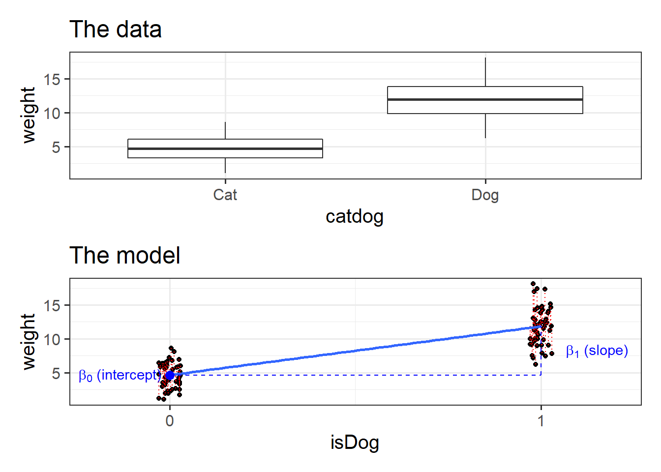
Figure 1: Binary Predictors
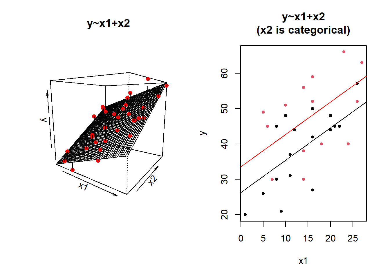
We can have categorical predictors in multiple regression, and not a great deal changes. Last week we visualised a regression surface, and if we have a binary predictor, instead of the continuum, we simply have two lines:
Fit the multiple regression model below using lm(), and assign it to an object to store it in your environment.
\[
\textrm{Wellbeing} = b_0 + b_1 (\textrm{Outdoor Time}) + b_2 (\textrm{HasARoutine}) + \epsilon
\]
\(\hat b_0\) (the intercept) is the estimated average wellbeing score associated with zero hours of weekly outdoor time and zero in the routine variable.
For which group (routine vs no routine) does the intercept correspond?
Hint: looking at the summary() might help
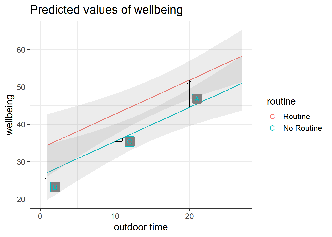
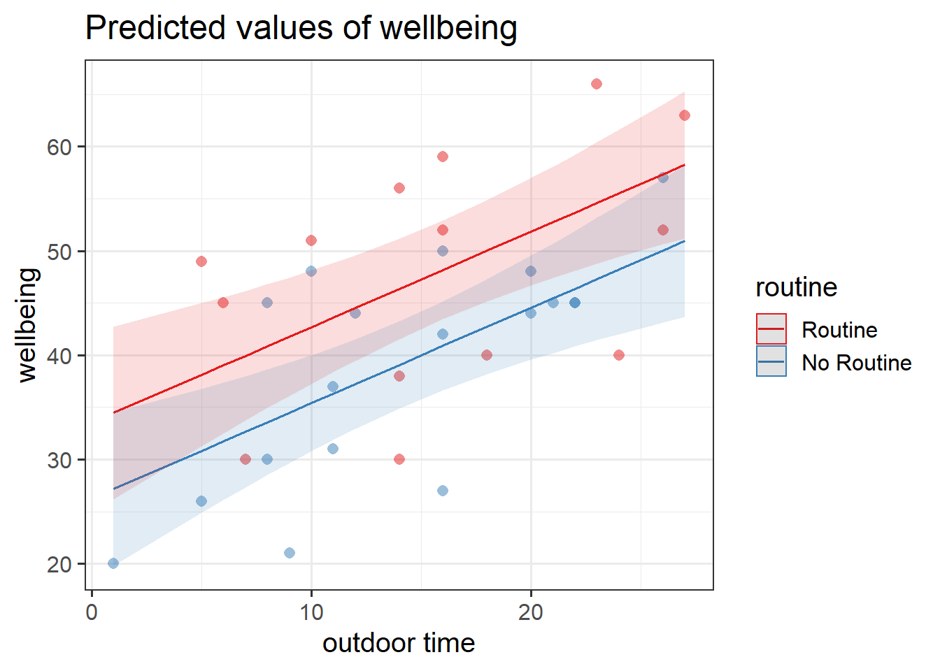
Get a pen and paper, and sketch out the plot shown in Figure 2.
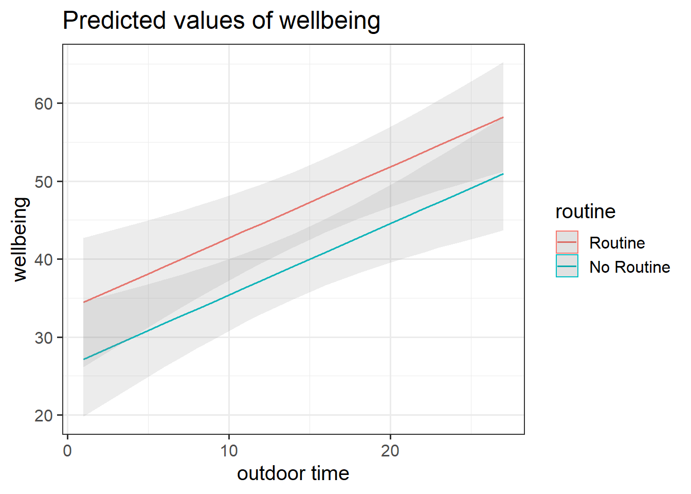
Figure 2: Multiple regression model: Wellbeing ~ Outdoor Time + Routine
Annotate your plot with labels for each of parameter estimates from your model:
| Parameter Estimate | Model Coefficient | Estimate |
|---|---|---|
| \(\hat b_0\) | (Intercept) |
26.25 |
| \(\hat b_1\) | outdoor_time |
0.92 |
| \(\hat b_2\) | routineRoutine |
7.29 |

Load the sjPlot package using library(sjPlot) and try running the code below (changing to use the name of your fitted model). You may already have the sjPlot package installed from previous exercises. If not, you will need to install it first.
library(sjPlot)
plot_model(wbmodel3)
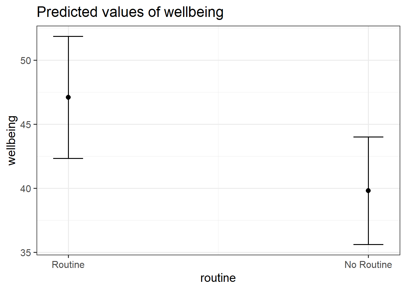
plot_model(wbmodel3, type = "pred")
plot_model(wbmodel3, type = "pred", terms=c("outdoor_time","routine"), show.data=TRUE)What do you think each one is showing?
The plot_model function (and the sjPlot package) can do a lot of different things. Most packages in R come with tutorials (or “vignettes”), for instance: https://strengejacke.github.io/sjPlot/articles/plot_model_estimates.html
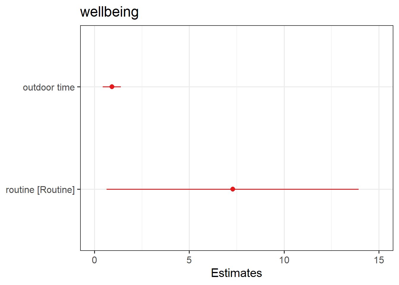 These are the parameter estimates (the
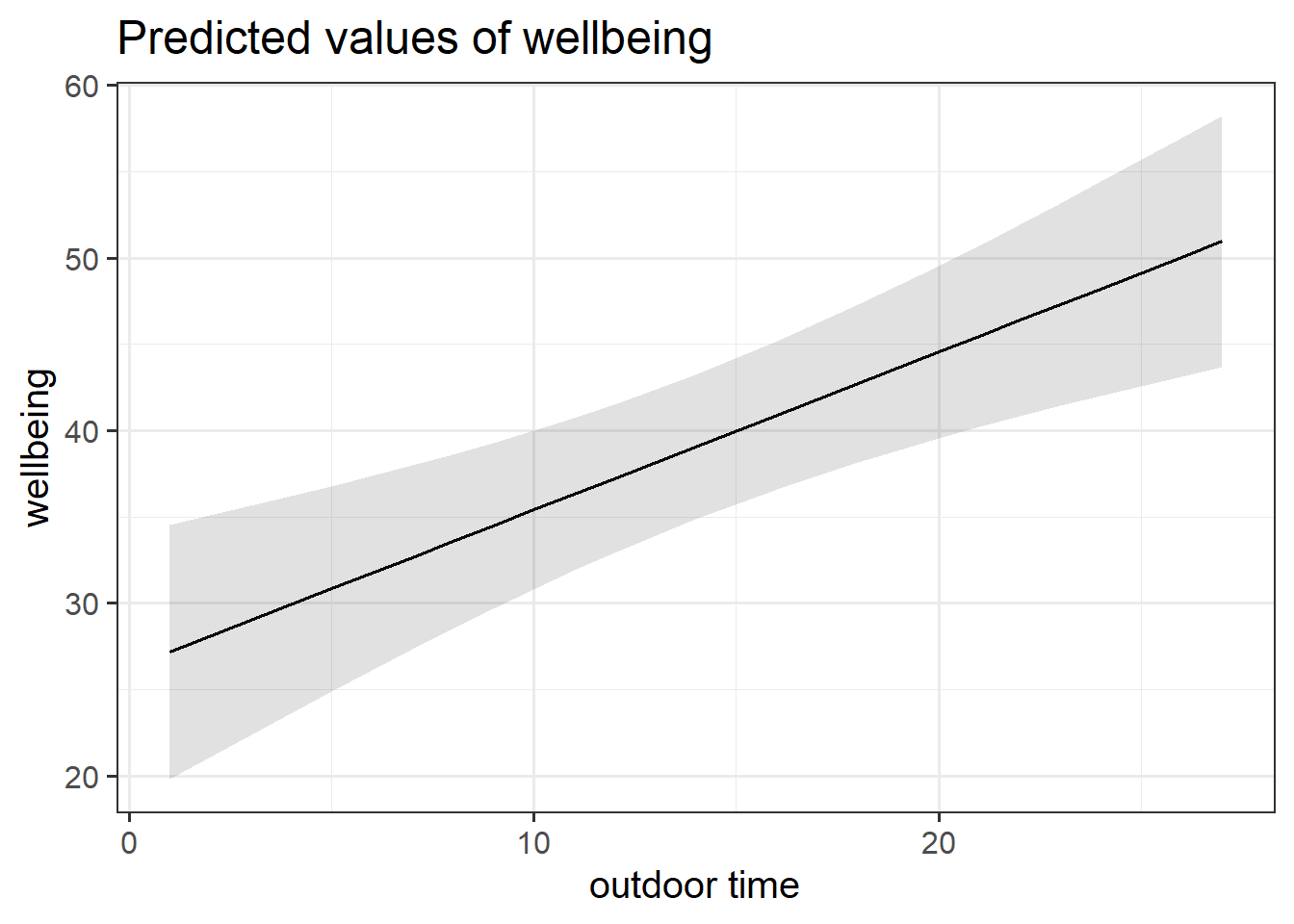
Categorical Predictors with \(k\) levels
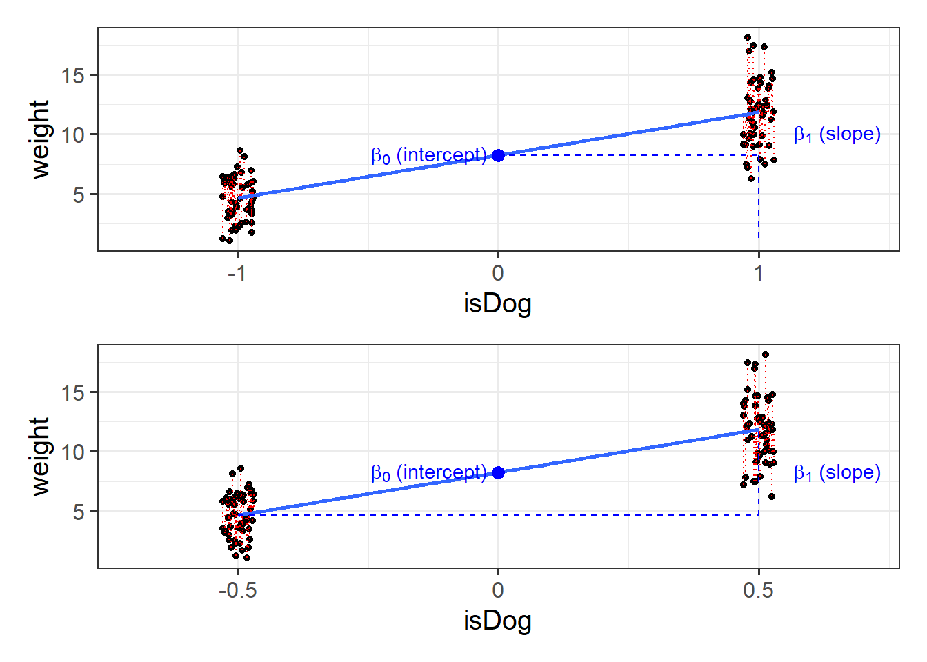
We have seen how a binary categorical variable gets inputted into our model as a variable of 0s and 1s (these typically get called “dummy variables”).
> Dummy variables are numeric variables that represent categorical data.
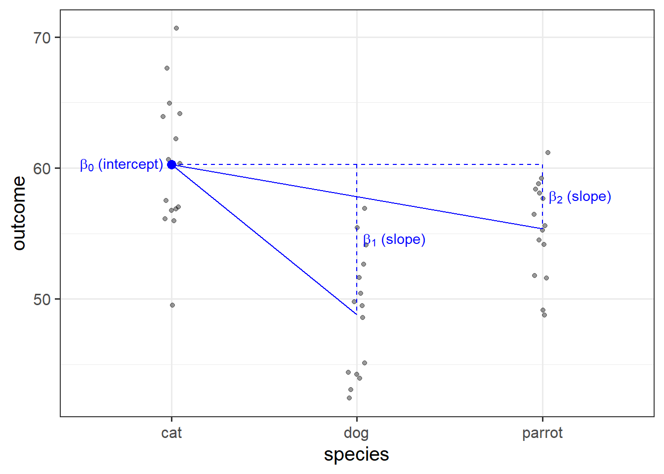
When we have a categorical explanatory variable with more than 2 levels, our model gets a bit bigger - it needs not just one, but a number of dummy variables. For a categorical variable with \(k\) levels, we can express it in \(k-1\) dummy variables.
For example, the “species” column below has three levels, and can be expressed by the two variables “species_dog” and “species_parrot”:
##   species species_dog species_parrot
## 1     cat           0              0
## 2     cat           0              0
## 3     dog           1              0
## 4  parrot           0              1
## 5     dog           1              0
## 6     cat           0              0
## 7 ... ... ...- The “cat” level is expressed whenever both the “species_dog” and “species_parrot” variables are 0.
- The “dog” level is expressed whenever the “species_dog” variable is 1 and the “species_parrot” variable is 0.
- The “parrot” level is expressed whenever the “species_dog” variable is 0 and the “species_parrot” variable is 1.
R will do all of this re-expression for us. If we include in our model a categorical explanatory variable with 4 different levels, the model will estimate 3 parameters - one for each dummy variable. We can interpret the parameter estimates (the coefficients we obtain using coefficients(),coef() or summary()) as the estimated increase in the outcome variable associated with an increase of one in each dummy variable (holding all other variables equal).
| Estimate | Std. Error | t value | Pr(>|t|) | |
|---|---|---|---|---|
| (Intercept) | 60.28 | 1.209 | 49.86 | 5.273e-39 |
| speciesdog | -11.47 | 1.71 | -6.708 | 3.806e-08 |
| speciesparrot | -4.916 | 1.71 | -2.875 | 0.006319 |
Note that in the above example, an increase in 1 of “species_dog” is the difference between a “cat” and a “dog.” An increase in one of “species_parrot” is the difference between a “cat” and a “parrot.” We think of the “cat” category in this example as the reference level - it is the category against which other categories are compared against.
If you think about it, a regression model with a categorical predictor with \(k\) levels is really just a regression model with \(k-1\) dummy variables as predictors.
Interactions
We’re now going to move on to something a little more interesting, and we’re finally going to stop using that dataset about wellbeing, outdoor time and socialising etc.
So far, we’ve been talking a lot about “the effect of x” and “change in y for a 1 unit change in x” etc. But what if we think that some such “effects” are actually dependent upon some other variable? For example, we might think that the amount to which caffeine makes you stressed depends upon how old you are.
An interaction is a quantitative researcher’s way of answering the question “what is the relationship between Y and X?” with, “well, it depends….”
We’re going to look at interactions between two numeric variables, but before that we’re going to look at an interaction between a numeric variable and a categorical variable.
~ Numeric * Categorical
Data: cogapoe.csv
Ninety adult participants were recruited for a study investigating how cognitive functioning varies by age, and whether this is different depending on whether people carry an APOE-4 gene.
cogapoe <- read_csv("../../data/cogapoe4.csv")
tibble(
  variables = names(cogapoe),
  description = c("Participant ID","Age (in Years)","Years of Education","Birthweight (in Kg)","APOE-4 Gene expansion ('none', 'apoe4a', 'apoe4b', apoe4c')","Score on Addenbrooke's Cognitive Examination")
) %>% knitr::kable() %>% kableExtra::kable_styling(.,full_width=T)| variables | description |
|---|---|
| pid | Participant ID |
| age | Age (in Years) |
| educ | Years of Education |
| birthweight_kg | Birthweight (in Kg) |
| apoe4 | APOE-4 Gene expansion (‘none,’ ‘apoe4a,’ ‘apoe4b,’ apoe4c’) |
| acer | Score on Addenbrooke’s Cognitive Examination |
Download Link
The data are available at https://uoepsy.github.io/data/cogapoe4.csv.
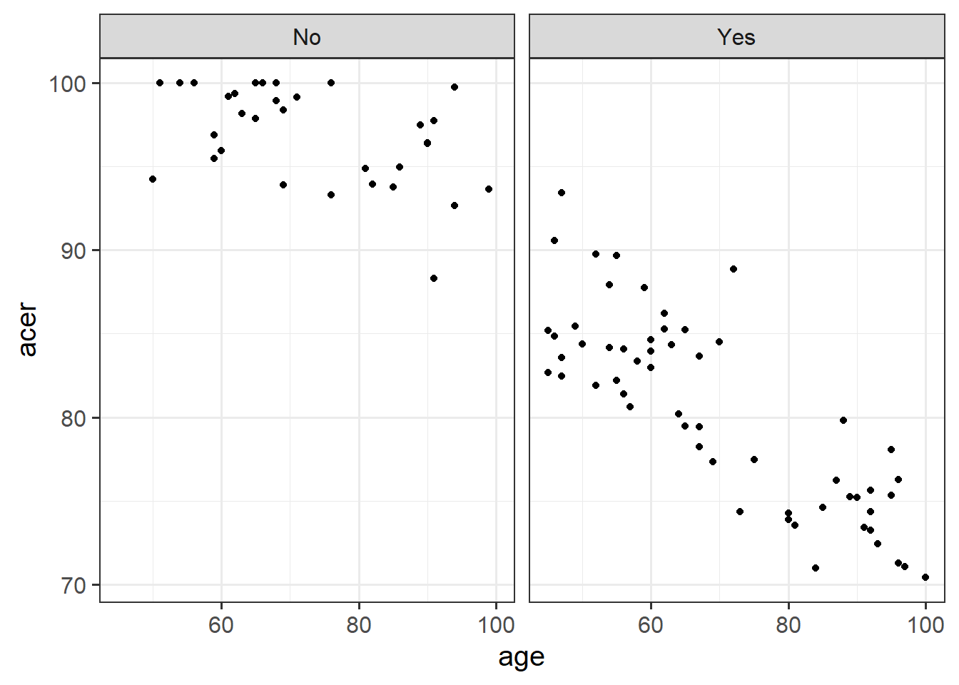
Research Question: Does the relationship between age and cognitive function differ between those with and without the APOE-4 genotype?
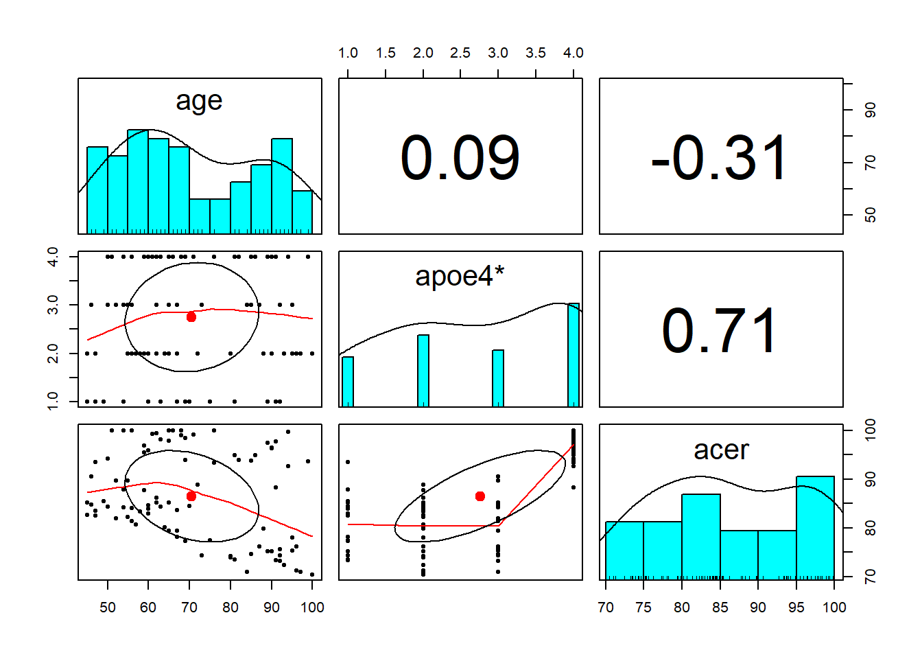
Read in the data and explore the variables which you think you will use to answer this research question (create some plots, some descriptive stats etc.)
Some tips:
- The
pairs.panels()function from the psych package is quite a nice way to plot a scatterplot matrix of a dataset.
- The
describe()function is also quite nice (from the psych package too).
Check the apoe4 variable. It currently has four levels (“none”/“apoe4a”/“apoe4b”/“apoe4c”), but the research question is actually interested in two (“none” vs “apoe4”). We’ll need to fix this. One way to do this would be to use ifelse() to define a variable which takes one value (e.g., “NO”) if the observation meets from some condition, or another value (e.g., “YES”) if it does not. Type ?ifelse in the console if you want to see the help function. You can use it to add a new variable either inside mutate(), or using data$new_variable_name <- ifelse(test, x, y) syntax. We saw it briefly in the previous set of exercises.
Produce a visualisation of the relationship between age and cognitive functioning, with separate facets for people with and without the APOE4 gene.
Hint: remember facet_wrap()?
Interactions in linear models
Specifying an interaction in a regression involves simply including the product of the two relevant predictor variables in your set of predictors. So if we are wanting to examine how the effect of \(x\) on \(y\) depends on \(z\), we would want to estimate a parameter \(b\) such that our outcome is predicted by \(b(x \times z)\). However, we also need to include \(x\) and \(z\) themselves: \(y = b_0 + b_1(x) + b_2(z) + b_3(x \times z)\).
“Except in special circumstances, a model including a product term for interaction between two explanatory variables should also include terms with each of the explanatory variables individually, even though their coefficients may not be significantly different from zero. Following this rule avoids the logical inconsistency of saying that the effect of \(X_1\) depends on the level of \(X_2\) but that there is no effect of \(X_1\).”
Ramsey and Schafer (2012)
To address the research question, we are going to fit the following model:
\[
\text{ACE-R} = b_0 + b_1(\text{Age}) + b_2(\text{isAPOE4}) + b_3 (\text{Age} \times \text{isAPOE4}) + \epsilon \\
\quad \\ \text{where} \quad \epsilon \sim N(0, \sigma) \text{ independently}
\]
Fit the model using lm().
Tip:
When fitting a regression model in R with two explanatory variables A and B, and their interaction, these two are equivalent:
- y ~ A + B + A:B
- y ~ A*B
Interpreting coefficients for A and B in the presence of an interaction A:B
When you include an interaction between \(x_1\) and \(x_2\) in a regression model, you are estimating the extent to which the effect of \(x_1\) on \(y\) is different across the values of \(x_2\).
What this means is that the effect of \(x_1\) on \(y\) depends on/is conditional upon the value of \(x_2\).
(and vice versa, the effect of \(x_2\) on \(y\) is different across the values of \(x_1\)).
This means that we can no longer talk about the “effect of \(x_1\) holding \(x_2\) constant.” Instead we can talk about a conditional effect of \(x_1\) on \(y\) at a specific value of \(x_2\).
When we fit the model \(y = b_0 + b_1(x_1)+ b_2(x_2) + b_3(x_1 \times x_2) + \epsilon\) using lm():
- the parameter estimate \(\hat b_1\) is the conditional effect of \(x_1\) on \(y\) where \(x_2 = 0\)
- the parameter estimate \(\hat b_2\) is the conditional effect of \(x_2\) on \(y\) where \(x_1 = 0\)
side note: Regardless of whether or not there is an interaction term in our model, all parameter estimates in multiple regression are “conditional” in the sense that they are dependent upon the inclusion of other variables in the model. For instance, in \(y = b_0 + b_1(x_1) + b_2(x_2) + \epsilon\) the coefficient \(\hat b_1\) is conditional upon holding \(x_2\) constant. The difference with an interaction is that they are conditional upon \(x_2\) being at some specific value.
Interpreting the interaction term A:B
The coefficient for an interaction term can be thought of as providing an adjustment to the slope.
In our model: \(\text{ACE-R} = b_0 + b_1(\text{Age}) + b_2(\text{isAPOE4}) + b_3 (\text{Age} \times \text{isAPOE4}) + \epsilon\), we have a numeric*categorical interaction.
The estimate \(\hat b_3\) is the adjustment to the slope \(\hat b_1\) to be made for the individuals in the \(\text{isAPOE4}=1\) group.
“The best method of communicating findings about the presence of significant interaction may be to present a table of graph of the estimated means at various combinations of the interacting variables.”
Ramsey and Schafer (2012)
Look at the parameter estimates from your model, and write a description of what each one corresponds to on the plot shown in Figure 3 (it may help to sketch out the plot yourself and annotate it).
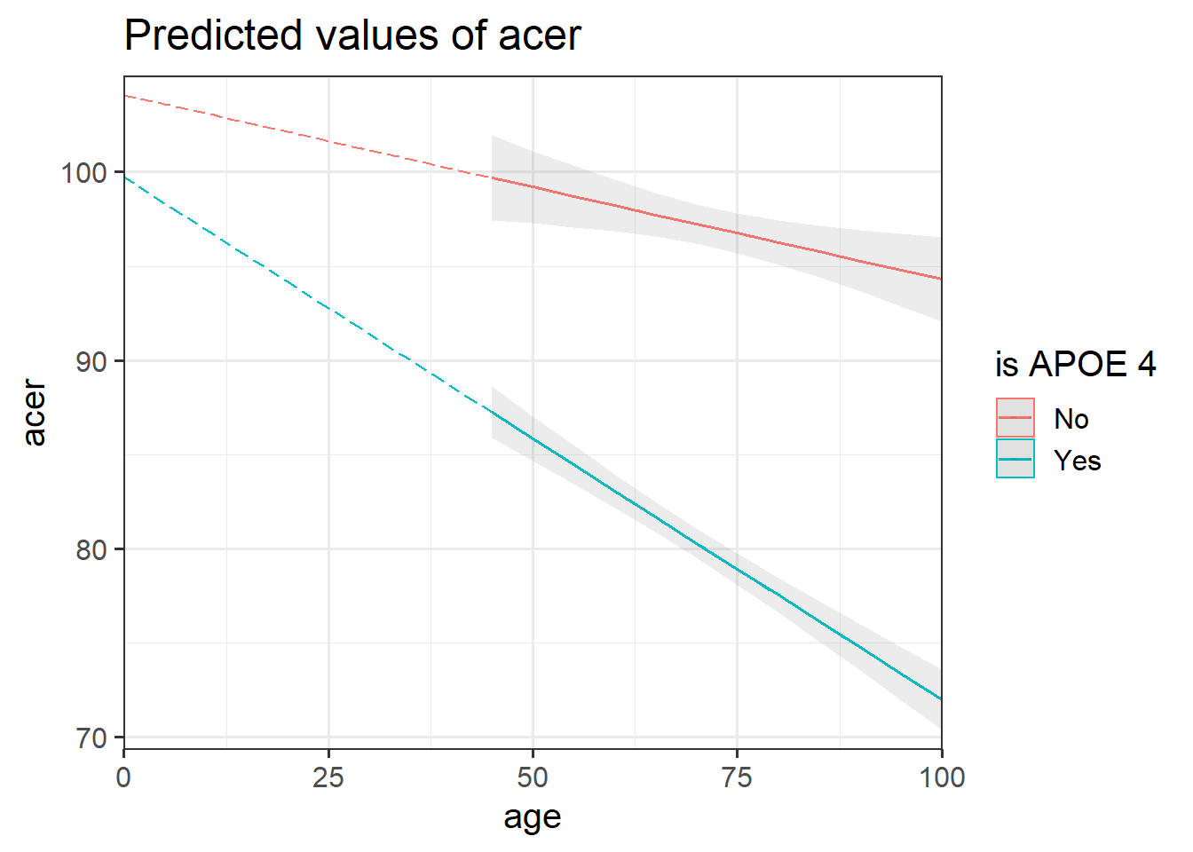
Figure 3: Multiple regression model: ACER ~ Age * isAPOE4
The dotted lines show the extension back to where the x-axis is zero
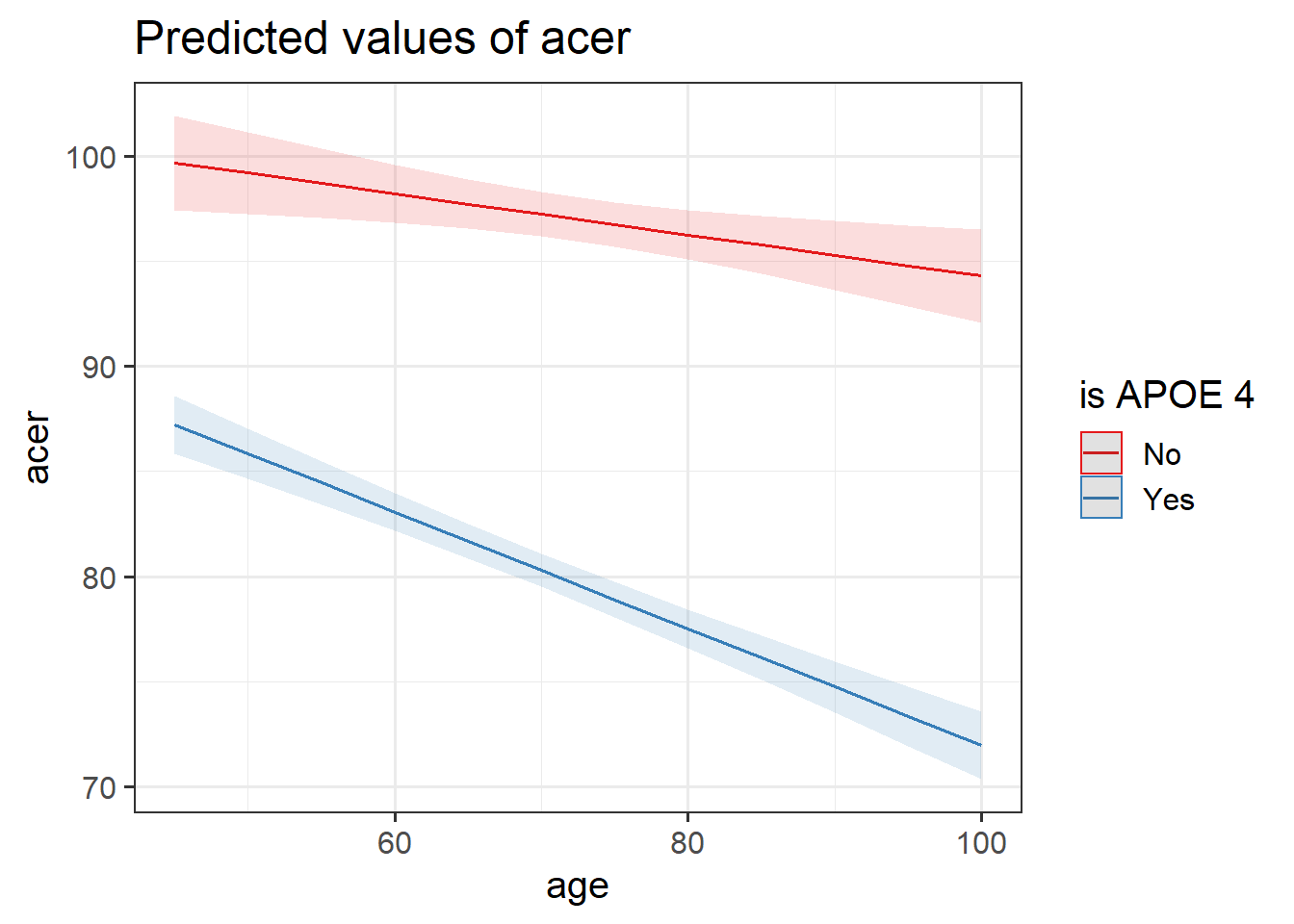
Make sure the sjPlot package is loaded and try using the function plot_model().
The default behaviour of plot_model() is to plot the parameter estimates and their confidence intervals. This is where type = "est".
Try to create a plot like Figure 3, which shows the two lines (Hint: what is this set block of exercises all about? type = ???.)
~ Numeric * Numeric
We will now look at a multiple regression model with an interaction between two numeric explanatory variables. For these exercises we’ll move onto another different dataset.
Data: scs_study.csv
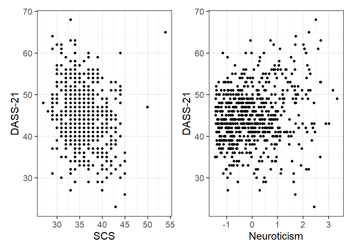
Data from 656 participants containing information on scores on each trait of a Big 5 personality measure, their perception of their own social rank, and their scores on a measure of depression.
The data in scs_study.csv contain seven attributes collected from a random sample of \(n=656\) participants:
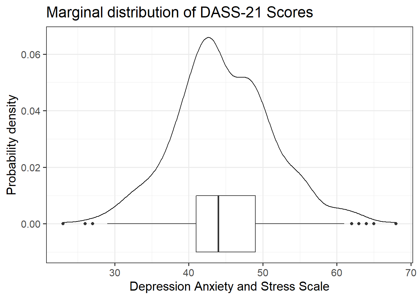
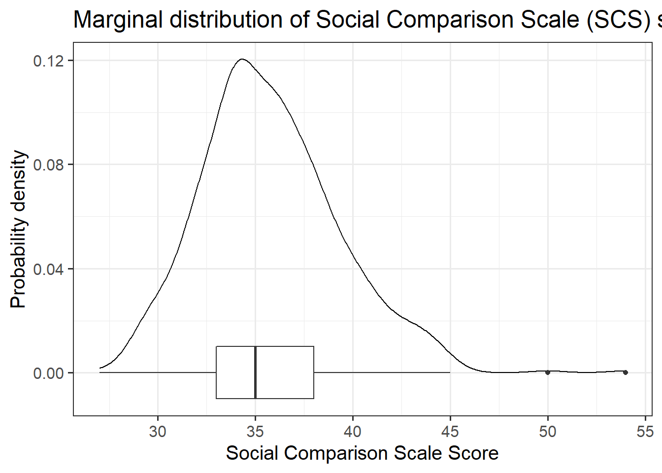
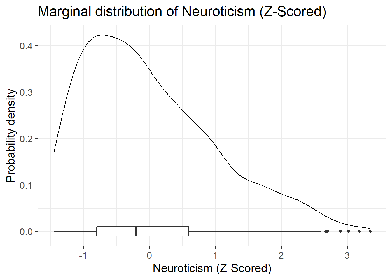
zo: Openness (Z-scored), measured on the Big-5 Aspects Scale (BFAS)zc: Conscientiousness (Z-scored), measured on the Big-5 Aspects Scale (BFAS)ze: Extraversion (Z-scored), measured on the Big-5 Aspects Scale (BFAS)za: Agreeableness (Z-scored), measured on the Big-5 Aspects Scale (BFAS)zn: Neuroticism (Z-scored), measured on the Big-5 Aspects Scale (BFAS)scs: Social Comparison Scale - An 11-item scale that measures an individual’s perception of their social rank, attractiveness and belonging relative to others. The scale is scored as a sum of the 11 items (each measured on a 5-point scale), with higher scores indicating more favourable perceptions of social rank.dass: Depression Anxiety and Stress Scale - The DASS-21 includes 21 items, each measured on a 4-point scale. The score is derived from the sum of all 21 items, with higher scores indicating higher a severity of symptoms.
Download link
The data is available at https://uoepsy.github.io/data/scs_study.csv
Refresher: Z-scores
When we standardise a variable, we re-express each value as the distance from the mean in units of standard deviations. These transformed values are called z-scores.
To transform a given value \(x_i\) into a z-score \(z_i\), we simply calculate the distance from \(x_i\) to the mean, \(\bar{x}\), and divide this by the standard deviation, \(s\):
\[
z_i = \frac{x_i - \bar{x}}{s}
\]
A Z-score of a value is the number of standard deviations below/above the mean that the value falls.
Research question
Previous research has identified an association between an individual’s perception of their social rank and symptoms of depression, anxiety and stress. We are interested in the individual differences in this relationship.
Specifically: Does the effect of social comparison on symptoms of depression, anxiety and stress vary depending on level of neuroticism?
Read in the Social Comparison Study data and explore the relevant distributions and relationships between the variables of interest to the research question.
Specify the model you plan to fit in order to answer the research question (e.g., \(\text{??} = b_0 + b_1 (\text{??}) + .... + \epsilon\))
scs_study in our environment, but you will likely have named yours something different. Edit the code below accordingly to run it on your data.The code takes the dataset, and uses the
cut() function to add a new variable called “zn_group,” which is the “zn” variable split into 4 groups.Remember: we have re-assign this output as the name of the dataset (the scs_study <- bit at the beginning) to make these changes occur in our environment (the top-right window of Rstudio). If we didn’t have the first line, then it would simply print the output.
scs_study <-
  scs_study %>%
  mutate(
    zn_group = cut(zn, 4)
  )
We can see how it has split the “zn” variable by plotting the two against one another:
(Note that the levels of the new variable are named according to the cut-points).
ggplot(data = scs_study, aes(x = zn_group, y = zn)) +
  geom_point()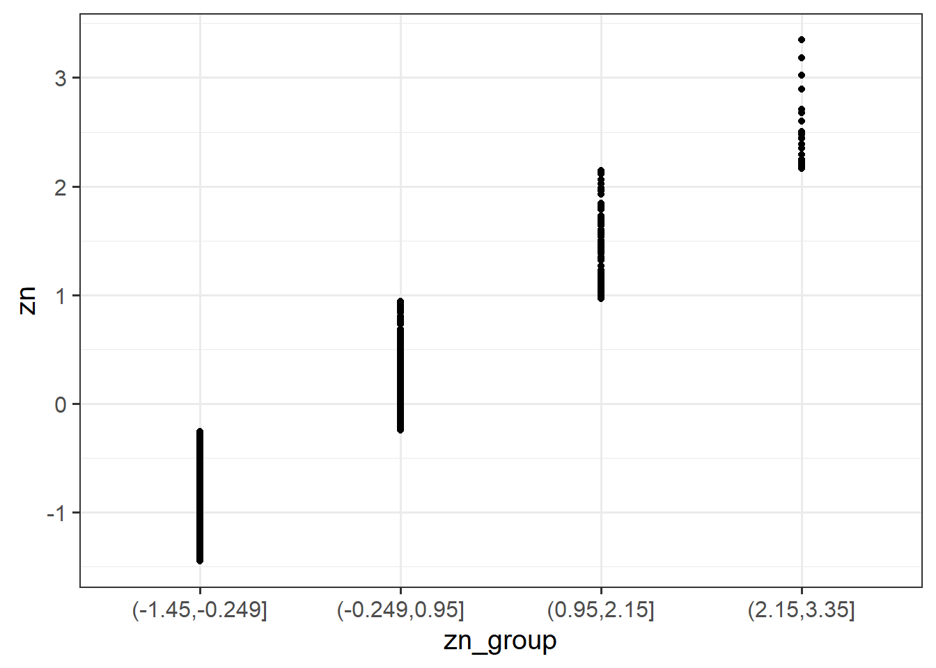
Plot the relationship between scores on the SCS and scores on the DASS-21, for each group of the variable (zn_group) that we just created.
How does the pattern change? Does it suggest an interaction?
Tip: Rather than creating four separate plots, you might want to map some feature of the plot to the variable we created in the data, or make use of facet_wrap()/facet_grid().
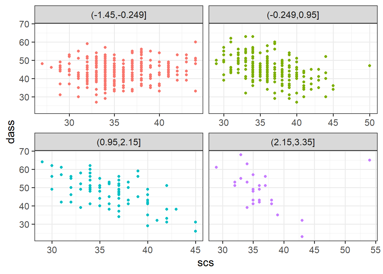
Cutting one of the explanatory variables up into groups essentially turns a numeric variable into a categorical one. We did this just to make it easier to visualise how a relationship changes across the values of another variable, because we can imagine a separate line for the relationship between SCS and DASS-21 scores for each of the groups of neuroticism. However, in grouping a numeric variable like this we lose information. Neuroticism is measured on a continuous scale, and we want to capture how the relationship between SCS and DASS-21 changes across that continuum (rather than cutting it into chunks).
We could imagine cutting it into more and more chunks (see Figure 4), until what we end up with is a an infinite number of lines - i.e., a three-dimensional plane/surface (recall that in for a multiple regression model with 2 explanatory variables, we can think of the model as having three-dimensions). The inclusion of the interaction term simply results in this surface no longer being necessarily flat. You can see this in Figure 5.
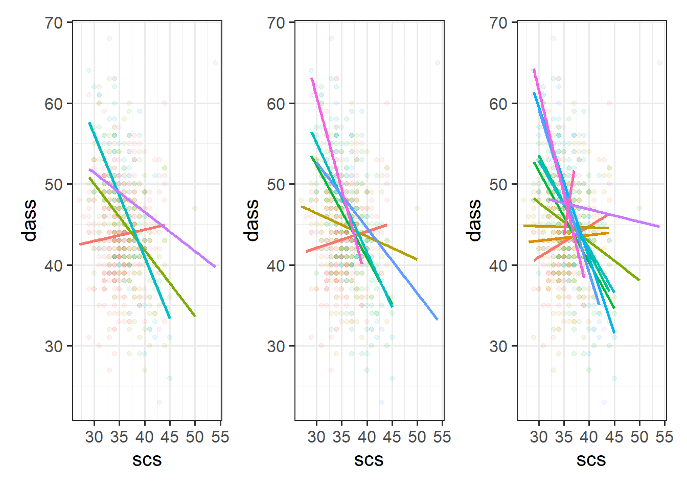
Figure 4: Separate regression lines DASS ~ SCS for neuroticism when cut into 4 (left) or 6 (center) or 12 (right) groups
Figure 5: 3D plot of regression surface with interaction. You can explore the plot in the figure below from different angles by moving it around with your mouse.
Fit your model using lm().
| Estimate | Std. Error | t value | Pr(>|t|) | |
|---|---|---|---|---|
| (Intercept) | 60.81 | 2.454 | 24.78 | 5.005e-96 |
| scs | -0.4439 | 0.06834 | -6.495 | 1.643e-10 |
| zn | 20.13 | 2.36 | 8.531 | 1.017e-16 |
| scs:zn | -0.5186 | 0.06552 | -7.915 | 1.063e-14 |
Recall that the coefficients zn and scs from our model now reflect the estimated change in the outcome associated with an increase of 1 in the explanatory variables, when the other variable is zero.
Think - what is 0 in each variable? what is an increase of 1? Are these meaningful? Would you suggest recentering either variable?
Recenter one or both of your explanatory variables to ensure that 0 is a meaningful value
We’ll now re-fit the model using mean-centered SCS scores instead of the original variable. Here are the parameter estimates:
dass_mdl2 <- lm(dass ~ 1 + scs_mc * zn, data = scs_study)

# pull out the coefficients from the summary():
summary(dass_mdl2)$coefficients
## Estimate Std. Error t value Pr(>|t|)
## (Intercept) 44.9324476 0.24052861 186.807079 0.000000e+00
## scs_mc -0.4439065 0.06834135 -6.495431 1.643265e-10
## zn 1.5797687 0.24086372 6.558766 1.105118e-10
## scs_mc:zn -0.5186142 0.06552100 -7.915236 1.063297e-14Fill in the blanks in the statements below.
- For those of average neuroticism and who score average on the SCS, the estimated DASS-21 Score is ???
- For those who who score ??? on the SCS, an increase of ??? in neuroticism is associated with a change of 1.58 in DASS-21 Scores
- For those of average neuroticism, an increase of ??? on the SCS is associated with a change of -0.44 in DASS-21 Scores
- For every increase of ??? in neuroticism, the change in DASS-21 associated with an increase of ??? on the SCS is asjusted by ???
- For every increase of ??? in SCS, the change in DASS-21 associated with an increase of ??? in neuroticism is asjusted by ???
What do we get when we use the plot_model() function from sjPlot to plot this continuous*continuous interaction?
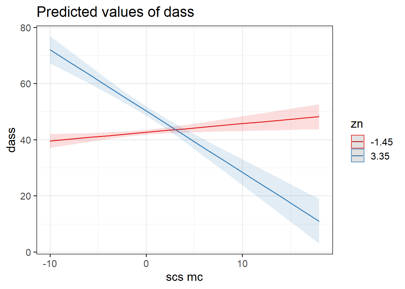 We might want to choose some other values, such as the mean of
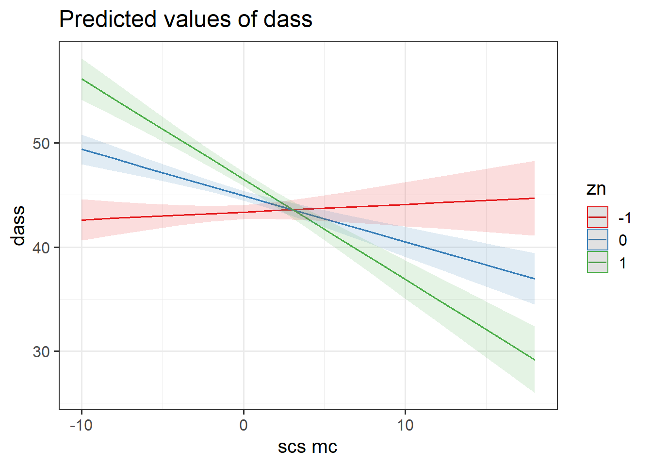
References
A common alternative is to use \(\beta\) for the population parameter, \(\hat \beta\) for the fitted estimate, and something like \(\hat \beta^*\) for the standardised estimate.↩︎

This workbook was written by Josiah King, Umberto Noe, and Martin Corley, and is licensed under a Creative Commons Attribution 4.0 International License.