Week 3 Exercises: Non-Linear Change

Cognitive Task Performance

Dataset: Az.rda

These data are available at https://uoepsy.github.io/data/Az.rda. You can load the dataset using:

load(url("https://uoepsy.github.io/data/Az.rda"))

and you will find the Az object in your environment.

The Az object contains information on 30 Participants with probable Alzheimer’s Disease, who completed 3 tasks over 10 time points: A memory task, and two scales investigating ability to undertake complex activities of daily living (cADL) and simple activities of daily living (sADL). Performance on all of tasks was calculated as a percentage of total possible score, thereby ranging from 0 to 100.

We’re interested in whether performance on these tasks differed at the outset of the study, and if they differed in their subsequent change in performance.

variable	description
Subject	Unique Subject Identifier
Time	Time point of the study (1 to 10)
Task	Task type (Memory, cADL, sADL)
Performance	Score on test (range 0 to 100)

Question 1

Load in the data and examine it.
How many participants, how many observations per participant, per task?

Solution 1.

load(url("https://uoepsy.github.io/data/Az.rda"))
summary(Az)

    Subject         Time          Task      Performance   
 1      : 30   Min.   : 1.0   cADL  :300   Min.   : 2.00  
 2      : 30   1st Qu.: 3.0   sADL  :300   1st Qu.:40.00  
 3      : 30   Median : 5.5   Memory:300   Median :52.00  
 4      : 30   Mean   : 5.5                Mean   :49.27  
 5      : 30   3rd Qu.: 8.0                3rd Qu.:61.00  
 6      : 30   Max.   :10.0                Max.   :85.00  
 (Other):720                                              

30 participants:

length(unique(Az$Subject))

[1] 30

Does every participant have 10 datapoints for each Task type? Yes!

any( table(Az$Subject, Az$Task) != 10 )

[1] FALSE

Question 2

No modelling just yet.

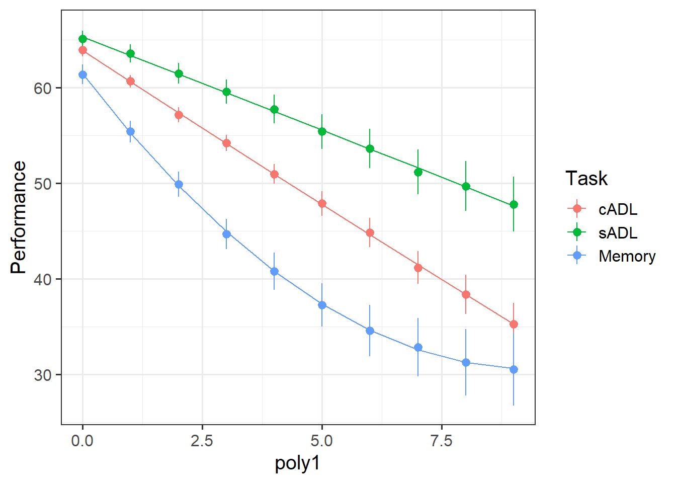
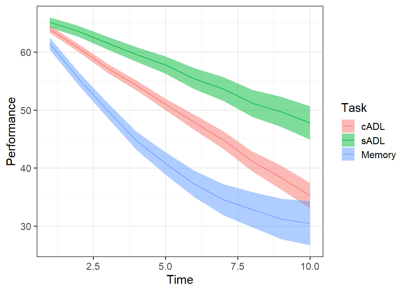
Plot the performance over time for each type of task.

Try using stat_summary so that you are plotting the means (and standard errors) of each task, rather than every single data point. Why? Because this way you can get a shape of the average trajectories of performance over time in each task.

Hints

For an example plot, see Chapter 6: polynomial growth #example-in-mlm.

Solution 2. You can use “pointranges”, or “line” and “ribbon”.
stat_summary will take the data and for each value of x calculate some function (in this case the mean, or the mean and SE):

ggplot(Az, aes(Time, Performance, color=Task, fill=Task)) + 
  stat_summary(fun.data=mean_se, geom="ribbon", color=NA, alpha=0.5) +
  stat_summary(fun=mean, geom="line")

Question 3

Why do you think raw/natural polynomials might be more useful than orthogonal polynomials for these data?

Hints

Are we somewhat interested in group differences (i.e. differences in scores, or differences in rate of change) at a specific point in time?

Solution 3. Because we’re interested in whether there are task differences at the starting point, raw polynomials are probably what we want here.

Question 4

Re-center the Time variable so that the intercept is the first timepoint.

Then choose an appropriate degree of polynomial (if any), and fit a full model that allows us to address the research aims.

Hints

Note there is no part of the research question that specifically asks about how “gradual” or “quick” the change is (which would suggest we are interested in the quadratic term).

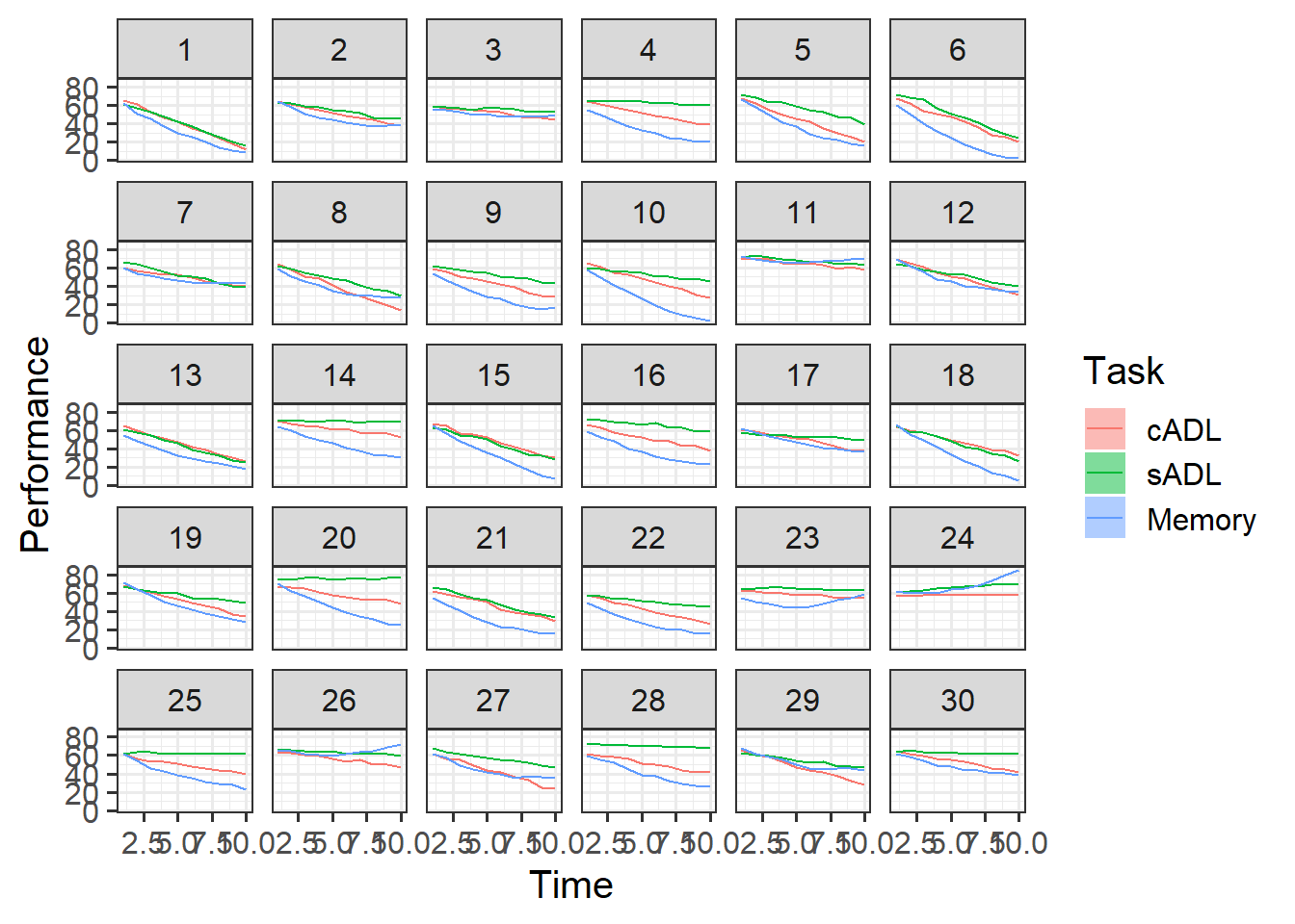
However, plots (summarised at the task level, and of individual participant’s data separately) can help to give us a sense of what degree of polynomial terms might be suitable to succinctly describe the trends.

In many cases, fitting higher and higher order polynomials will likely result in a ‘better fit’ to our sample data, but these will be worse and worse at generalising to new data - i.e. we run the risk of overfitting.

Solution 4. In our plot, there were 2 straight line and one slightly curvy one. It wasn’t S-shaped or ‘wiggly’ or anything, there was just a bit of a bend in it, which suggests that the quadratic term could be a good approximation here.

It’s worth also looking at the individual participant trajectories. In these we can also see the curvi-ness of the blue line - it’s more pronounced for some people than others, but it does seem like individual’s trajectories on the Memory task may be curvilinear.

ggplot(Az, aes(Time, Performance, color=Task, fill=Task)) + 
  stat_summary(fun.data=mean_se, geom="ribbon", color=NA, alpha=0.5) +
  stat_summary(fun=mean, geom="line")+
  facet_wrap(~Subject)

library(lme4)
Az <- Az |> mutate(
  Time1 = Time-1,
  poly1 = poly(Time1,2,raw=T)[,1],
  poly2 = poly(Time1,2,raw=T)[,2]
)

Or using Dan’s code:

# import Dan's code:
source("https://uoepsy.github.io/msmr/functions/code_poly.R")

# this also produces a nice little plot to show the polynomials
Az$Time1 <- Az$Time-1
Az <- code_poly(df = Az, predictor = 'Time1',
                poly.order = 2, orthogonal = FALSE)

Solution 5. We’re interested in how performance changes over time, but we have poly1 and poly2 for time, so we’re at:

lmer(Performance ~ poly1 + poly2 ... 

Our research aims are to investigate differences between task performance (both at baseline and change over time). So we want to interact time with task:

lmer(Performance ~ (poly1 + poly2)*Task ... 

Solution 6.

head(Az)

  Subject Time Task Performance Time1 poly1 poly2
1       1    1 cADL          65     0     0     0
2       1    2 cADL          61     1     1     1
3       1    3 cADL          53     2     2     4
4       1    4 cADL          46     3     3     9
5       1    5 cADL          42     4     4    16
6       1    6 cADL          35     5     5    25

We have 900 observations, and 30 for each participant.

lmer(Performance ~ (poly1 + poly2)*Task ... +
                   (1 + .... | Subject)

Fixed vs Random

We can account for group differences in models either by estimating group differences, or by estimating variance between groups:

• group as a fixed effect (y ~ 1 + group) = groups differ in \(y\) by \(b_1, b_2, ..., b_k\)
  
• group as a random effect (y ~ 1 + (1|group)) = groups vary in \(y\) with a standard deviation of \(\sigma_0\)

One way to think about whether a group is best in the random effects part or in the fixed part of our model is to think about “what would happen if I repeated the experiment?”

Should variable g be fixed or random?

	Repetition: If the experiment were repeated:	Desired inference: The conclusions refer to:
Fixed \(y\,\sim\,~\,...\, +\, g\)	Same groups would be used	The groups used
Random \(y\,\sim\,...\,+\,(\,... |\,g)\)	Different groups would be used	A population from which the groups used are just a (random) sample

Practical points:
- Sometimes there isn’t enough variability between groups to model as random effects (i.e. the variance gets estimated as too close to zero). - Sometimes you might not have sufficient number of groups to model as random effects (e.g. for groups of fewer than c8 things, estimates of the variance are often not a reliable reflection of the population).

Solution 7. What slopes could vary by participant?

Q: Could participants vary in their performance over time?
A: Yes, (poly1 + poly2 | Subject)
Q: Could participants vary in how performance differs between Tasks?
A: Yes, (poly1 + poly2 + Task | Subject). E.g., Some participants might be much better at the memory task than other tasks, some might be better at the other tasks.
Q: Could participants vary in how tasks differ in their performance over time?
A: Yes, ((poly1 + poly2)*Task | Subject). E.g., For some participants, memory could decline more than cADL, for other participants it could decline less.

lmer(Performance ~ (poly1 + poly2)*Task ... +
                   (1 + (poly1 + poly2)*Task | Subject)

Solution 8. small note: I’m using the bobyqa optimizer here because it tends to be slightly quicker than the default.

m1 = lmer(Performance ~ (poly1 + poly2) * Task +
            (1 + (poly1 + poly2) * Task | Subject),
          data=Az, control=lmerControl(optimizer = "bobyqa"))

boundary (singular) fit: see help(‘isSingular’)
Warning messages:
1: In commonArgs(par, fn, control, environment()) :
maxfun < 10 * length(par)^2 is not recommended.
2: In optwrap(optimizer, devfun, getStart(start, rho$pp), lower = rho$lower, :
convergence code 1 from bobyqa: bobyqa – maximum number of function evaluations exceeded

Question 5

Okay, so the model didn’t converge. It’s trying to estimate a lot of things in the random effects (even though it didn’t converge, try looking at VarCorr(model) to see all the covariances it is trying to estimate).

Categorical random effects on the RHS

When we have a categorical random effect (i.e. where the x in (1 + x | g) is a categorical variable), then model estimation can often get tricky, because “the effect of x” for a categorical variable with \(k\) levels is identified via \(k-1\) parameters, meaning we have a lot of variances and covariances to estimate when we include x|g.

When x is numeric:

Groups   Name        Std.Dev. Corr  
g        (Intercept) ...        
         x           ...      ...
Residual             ...     

When x is categorical with \(k\) levels:

Groups   Name        Std.Dev. Corr  
g        (Intercept) ...        
         xlevel2     ...      ...
         xlevel3     ...      ...     ...
         ...         ...      ...     ...     ...
         xlevelk     ...      ...     ...     ...   ...
Residual             ...     

However, we can use an alternative formation of the random effects by putting a categorical x into the right-hand side:
Instead of (1 + x | g) we can fit (1 | g) + (1 | g:x).

The symbol : in g:x is used to refer to the combination of g and x.

      g        x     g:x
1    p1        a    p1.a
2    p1        a    p1.a
3    p1        b    p1.b
4   ...      ...     ...
5    p2        a    p2.a
6    p2        b    p2.b
7   ...      ...     ...

It’s a bit weird to think about it, but these two formulations of the random effects can kind of represent the same idea:

• (1 + x | g): each group of g can have a different intercept and a different effect of x
  
• (1 | g) + (1 | g:x): each group of g can have a different intercept, and each level of x within each g can have a different intercept.

Both of these allow the outcome y to change across x differently for each group in g (i.e. both of them result in y being different for each level of x in each group g).
The first does so explicitly by estimating the group level variance of the y~x effect.
The second one estimates the variance of \(y\) between groups, and also the variance of \(y\) between ‘levels of x within groups’. In doing so, it achieves more or less the same thing, but by capturing these as intercept variances between levels of x, we don’t have to worry about lots of covariances:

(1 + x | g)

Groups   Name        Std.Dev. Corr  
g        (Intercept) ...        
         xlevel2     ...      ...
         xlevel3     ...      ...     ...
         ...         ...      ...     ...     ...
         xlevelk     ...      ...     ...     ...   ...
Residual             ...     

(1 | g) + (1 | g:x)

Groups   Name        Std.Dev. 
g        (Intercept) ...        
g.x      (Intercept) ...        
Residual             ...     

Try adjusting your model by first moving Task to the right hand side of the random effects, and from there starting to simplify things (remove random slopes one-by-one)

This is our first experience of our random effect structures becoming more complex than simply (.... | group). This is going to feel confusing, but don’t worry, we’ll see more structures like this next week.

Hints

... + (1 + poly1 + poly2 | Subject) + (1 + poly1 + poly2 | Subject:Task)

To then start simplifying (if this model doesn’t converge), it can be helpful to look at the VarCorr() of the non-converging model to see if anything looks awry. Look for small variances, perfect (or near perfect) correlations. These might be sensible things to remove.

Solution 9. Here’s our model with subject-task effects on the right hand side.
Again we have problems, as we have a singular fit:

m2 = lmer(Performance ~ (poly1 + poly2) * Task +
            (1 + poly1 + poly2 | Subject) +
            (1 + poly1 + poly2 | Subject:Task),
          data=Az, control=lmerControl(optimizer = "bobyqa"))

boundary (singular) fit: see help(‘isSingular’)

Looking at the random effects of our model, note that the poly2|Subject random effect has very little variance (and high correlations).
Note that it makes sense that by including the random effects for Subject:Task, there might not be much above that leftover in Subject random effects.

VarCorr(m2)

 Groups       Name        Std.Dev. Corr         
 Subject:Task (Intercept) 3.100837              
              poly1       0.923485  0.275       
              poly2       0.052644 -0.329  0.021
 Subject      (Intercept) 3.461349              
              poly1       1.565908 -0.177       
              poly2       0.007638  0.075 -0.995
 Residual                 1.019574              

When we remove it, our model converges!!

m3 = lmer(Performance ~ (poly1 + poly2) * Task +
            (1 + poly1 | Subject) +
            (1 + poly1 + poly2 | Subject:Task),
          data=Az, control=lmerControl(optimizer = "bobyqa"))

Question 6

Conduct a series of model comparisons investigating whether

1. Tasks differ only in their linear change
   
2. Tasks differ in their quadratic change

Hints

Remember, these sorts of model comparisons are being used to isolate and test part of the fixed effects (we’re interested in the how the average participant performs over the study). So our models want to have the same random effect structure, but different fixed effects.

See the end of Chapter 6: polynomial growth #example-in-mlm.

Solution 10. As I’m comparing these with a likelihood ratio test, I’ll fit them with REML=FALSE

m3int = lmer(Performance ~ poly1 + poly2 + Task + 
            (1 + poly1 | Subject) +
            (1 + poly1 + poly2 | Subject:Task),
            REML = FALSE,
          data=Az, control=lmerControl(optimizer = "bobyqa"))

m3lin = lmer(Performance ~ poly1*Task + poly2 +
            (1 + poly1 | Subject) +
            (1 + poly1 + poly2 | Subject:Task),
            REML = FALSE,
          data=Az, control=lmerControl(optimizer = "bobyqa"))

m3full = lmer(Performance ~ (poly1 + poly2) * Task +
            (1 + poly1 | Subject) +
            (1 + poly1 + poly2 | Subject:Task),
            REML = FALSE,
          data=Az, control=lmerControl(optimizer = "bobyqa"))

anova(m3int, m3lin, m3full)

Data: Az
Models:
m3int: Performance ~ poly1 + poly2 + Task + (1 + poly1 | Subject) + (1 + poly1 + poly2 | Subject:Task)
m3lin: Performance ~ poly1 * Task + poly2 + (1 + poly1 | Subject) + (1 + poly1 + poly2 | Subject:Task)
m3full: Performance ~ (poly1 + poly2) * Task + (1 + poly1 | Subject) + (1 + poly1 + poly2 | Subject:Task)
       npar    AIC    BIC  logLik deviance   Chisq Df Pr(>Chisq)    
m3int    15 3801.8 3873.8 -1885.9   3771.8                          
m3lin    17 3775.4 3857.0 -1870.7   3741.4  30.413  2  2.488e-07 ***
m3full   19 3607.8 3699.1 -1784.9   3569.8 171.532  2  < 2.2e-16 ***
---
Signif. codes:  0 '***' 0.001 '**' 0.01 '*' 0.05 '.' 0.1 ' ' 1

The linear change over time differs between Tasks (\(\chi^2(2) = 30.41, p < 0.001). The quadratic change over time differs between Tasks (\)^2(2) = 171.53, p < 0.001).

Question 7

Get some confidence intervals and provide an interpretation of each coefficient from the full model.

Solution 11. As we’ve used likelihood ratio tests above, we’ll get some profile likelihood confidence intervals for our parameters.
note this took me about 4 mins to run
If you want to get some quicker (slightly less robust) confidence intervals, then switch "profile" to "Wald".

confint(m3full, method="profile", parm="beta_")

term	est	CI	interpretation
(Intercept)	63.88	[62.19, 65.57]	estimated score on the cADL task at baseline
poly1	-3.27	[-3.93, -2.61]	estimated linear change in cADL scores from baseline
poly2	0.01	[-0.02, 0.03]	no significant curvature to the cADL trajectory
TasksADL	1.44	[-0.18, 3.06]	no significant difference between sADL and cADL tasks at baseline
TaskMemory	-2.40	[-4.02, -0.78]	at baseline, scores on memory task are 2.4 lower than cADL
poly1:TasksADL	1.34	[0.82, 1.85]	performance on sADL task is not decreasing from baseline as much as performance on cADL
poly1:TaskMemory	-3.30	[-3.81, -2.78]	performance on Memory task is decreasing (linearly) more than performance on cADL
poly2:TasksADL	-0.01	[-0.05, 0.02]	no significant difference between quadratic change of sADL from that of cADL
poly2:TaskMemory	0.34	[0.3, 0.37]	significant difference in quadratic change between performance on Memory vs performance on cADL

some tables of predictions (in case they help)

To get a sense of the quadratic term ‘in action’, think about the predictions across time for each task:

For cADL, this is just the linear change. Every timepoint, performance decreases by 3.27.

timepoint	cADL
prediction formula	\(63.88 + (-3.27 \times time) + (0.01 \times time^2)\)
prediction formula (with non-sig terms removed)	\(63.88 + (-3.27 \times time)\)
0	\(63.88 + (-3.27 \times 0) = 63.88\)
1	\(63.88 + (-3.27 \times 1) = 60.61\)
2	\(63.88 + (-3.27 \times 2) = 57.34\)
3	\(63.88 + (-3.27 \times 3) = 54.07\)

For sADL, the additional change is +1.34, so at every timepoint performance decreases by -1.93 (this is -3.27+1.34)

timepoint	sADL
prediction formula	\(63.88 + (-3.27 \times time) + (0.01 \times time^2) +\) \((1.44) + (1.34 \times time) + (-0.01 \times time^2)\)
prediction formula (with non-sig terms removed)	\(63.88 + (-3.27 \times time) + (1.34 \times time)\)
0	\(63.88 + (-3.27 \times 0) + (1.34 \times 0) = 63.88\)
1	\(63.88 + (-3.27 \times 1) + (1.34 \times 1) = 61.95\)
2	\(63.88 + (-3.27 \times 2)+ (1.34 \times 2) = 60.02\)
3	\(63.88 + (-3.27 \times 3)+ (1.34 \times 3) = 58.09\)

For the Memory task, the quadratic term is in play. at every timepoint performance decreases by \(-3.27-3.30 +(0.34 \times time^2)\). So for low timepoints, the quadratic term doesn’t make much of a difference as it does for bigger time points.

timepoint	Memory
prediction formula	\(63.88 + (-3.27 \times time) + (0.01 \times time^2) +\) \((-2.40) + (-3.30 \times time) + (0.34 \times time^2)\)
prediction formula (with non-sig terms removed)	\(63.88 + (-3.27 \times time) +\) \((-2.40) + (-3.30 \times time) + (0.34 \times time^2)\)
0	\(63.88 + (-3.27 \times 0) +\) \((-2.40) + (-3.30 \times 0) + (0.34 \times 0^2) = 61.48\)
1	\(63.88 + (-3.27 \times 1) +\) \((-2.40) + (-3.30 \times 1) + (0.34 \times 1^2) = 55.25\)
2	\(63.88 + (-3.27 \times 2) +\) \((-2.40) + (-3.30 \times 2) + (0.34 \times 2^2) = 49.70\)
3	\(63.88 + (-3.27 \times 3) +\) \((-2.40) + (-3.30 \times 3) + (0.34 \times 3^2) = 44.83\)
…	…
9	\(63.88 + (-3.27 \times 9) +\) \((-2.40) + (-3.30 \times 9) + (0.34 \times 9^2) = 29.89\)
10	\(63.88 + (-3.27 \times 10) +\) \((-2.40) + (-3.30 \times 10) + (0.34 \times 10^2) = 29.78\)

Question 8

Take a piece of paper, and based on your interpretation for the previous question, sketch out the model estimated trajectories for each task.

Solution 12.

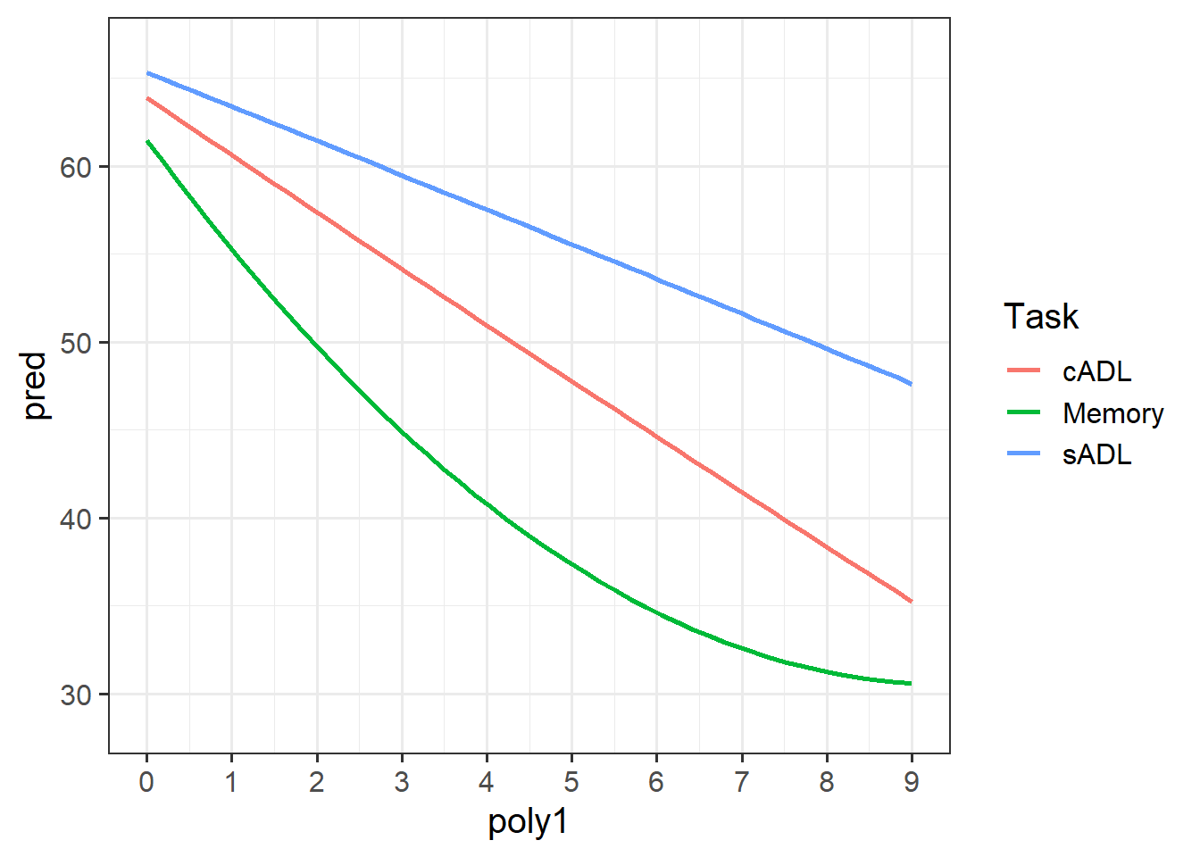
Question 9

Make a plot showing both the average performance and the average model predicted performance across time.

Solution 13.

library(broom.mixed)
augment(m3) |>
  ggplot(aes(x=poly1,col=Task))+
  stat_summary(aes(y=Performance), geom="pointrange") + 
  stat_summary(aes(y=.fitted), geom="line")