Week 1 Exercises: Intro to MLM

New Packages!

These are the main packages we’re going to use in this block. It might make sense to install them now if you do not have them already

• tidyverse : for organising data
  
• lme4 : for fitting generalised linear mixed effects models
• broom.mixed : tidying methods for mixed models
• effects : for tabulating and graphing effects in linear models
• lmerTest: for quick p-values from mixed models
• parameters: various inferential methods for mixed models

Getting to grips with MLM

These first set of exercises are not “how to do analyses with multilevel models” - they are designed to get you thinking, and help with an understanding of how these models work.

Data: New Toys!

Recall the example from last semesters’ USMR course, where the lectures explored linear regression with a toy dataset of how practice influences the reading age of toy characters (see USMR Week 7 Lecture). We’re going to now broaden our scope to the investigation of how practice affects reading age for all toys (not just Martin’s Playmobil characters).

You can find a dataset at https://uoepsy.github.io/data/toy2.csv containing information on 129 different toy characters that come from a selection of different families/types of toy. You can see the variables in the table below¹.

variable	description
toy_type	Type of Toy
year	Year Released
toy	Character
hrs_week	Hours of practice per week
R_AGE	Reading Age

Question 1

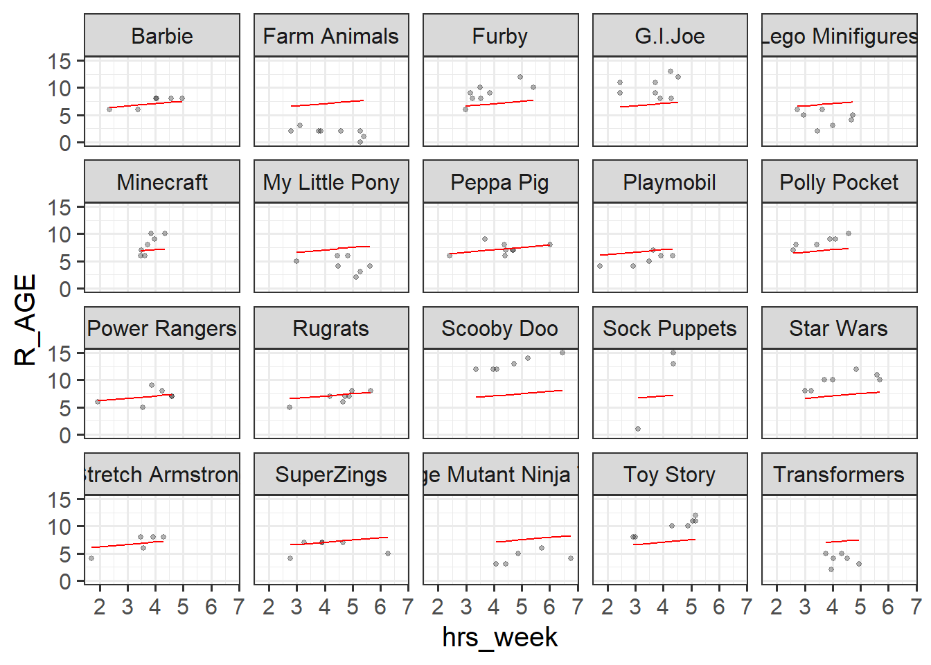
Below is some code that fits a model of “reading age” (R_AGE) predicted by hours of practice (hrs_week). Line 2 then gets the ‘fitted’ values from the model and adds them as a new column to the dataset, called pred_lm. The fitted values are what the model predicts for every individual observation (every individual toy in our dataset).

Lines 4-7 then plot the data, split up by each type of toy, and adds lines showing the model fitted values.

Run the code and check that you get a plot. What do you notice about the lines?

lm_mod <- lm(R_AGE ~ hrs_week, data = toy2)
toy2$pred_lm <- predict(lm_mod)

ggplot(toy2, aes(x = hrs_week)) + 
  geom_point(aes(y = R_AGE), size=1, alpha=.3) +
  facet_wrap(~toy_type) +
  geom_line(aes(y=pred_lm), col = "red")

Solution 1. We should get something like this:

lm_mod <- lm(R_AGE ~ hrs_week, data = toy2)
toy2$pred_lm <- predict(lm_mod)

ggplot(toy2, aes(x = hrs_week)) + 
  geom_point(aes(y = R_AGE), size=1, alpha=.3) +
  facet_wrap(~toy_type) +
  geom_line(aes(y=pred_lm), col = "red")

Note that the lines are exactly the same for each type of toy. This makes total sense, because the model (which is where we’ve got the lines from) completely ignores the toy_type variable!

Question 2

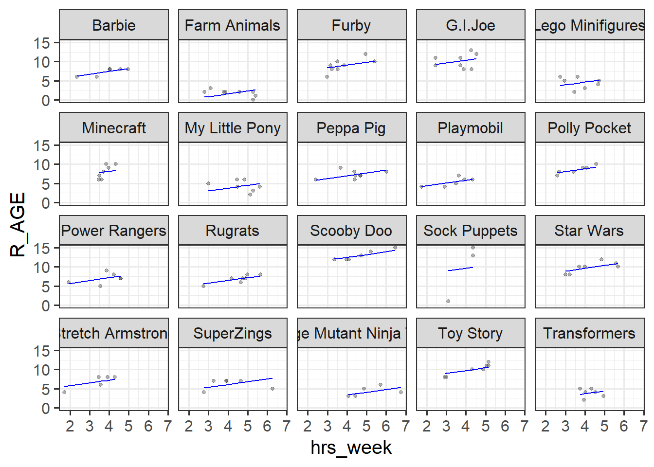
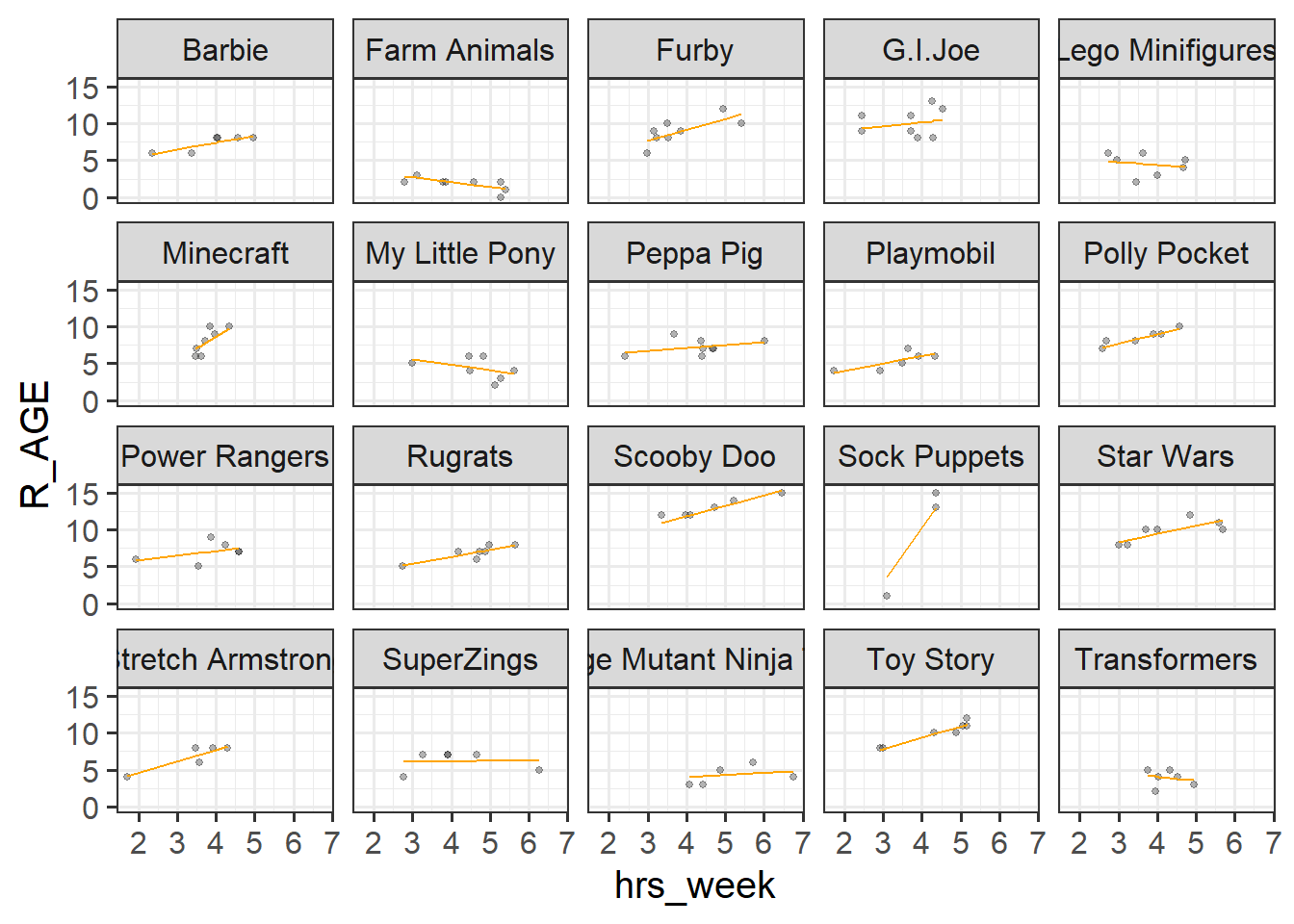
Below are 3 more code chunks that all 1) fit a model, then 2) add the fitted values of that model to the plot.

The first model is a ‘no-pooling’ approach, where we use tools learned in USMR and simply add in toy_type as a predictor in the model to estimate all the differences between types of toys.

The second and third are multilevel models. The second fits random intercepts by-toytype, and the third fits random intercepts and slopes of hrs_week

Copy each chunk and run through the code. Pay attention to how the lines differ.

fe_mod <- lm(R_AGE ~ toy_type + hrs_week, data = toy2)
toy2$pred_fe <- predict(fe_mod)

ggplot(toy2, aes(x = hrs_week)) + 
  geom_point(aes(y = R_AGE), size=1, alpha=.3) +
  facet_wrap(~toy_type) +
  geom_line(aes(y=pred_fe), col = "blue")

library(lme4)
ri_mod <- lmer(R_AGE ~ hrs_week + (1 | toy_type), data = toy2)
toy2$pred_ri <- predict(ri_mod)

ggplot(toy2, aes(x = hrs_week)) + 
  geom_point(aes(y = R_AGE), size=1, alpha=.3) +
  facet_wrap(~toy_type) +
  geom_line(aes(y=pred_ri), col = "green")

rs_mod <- lmer(R_AGE ~ hrs_week + (1 + hrs_week | toy_type), data = toy2)
toy2$pred_rs <- predict(rs_mod)

ggplot(toy2, aes(x = hrs_week)) + 
  geom_point(aes(y = R_AGE), size=1, alpha=.3) +
  facet_wrap(~toy_type) +
  geom_line(aes(y=pred_rs), col = "orange")

Solution 2. The first model has an adjustment for each toy-type (we can see this in the coefficients if we want). What this means is that the line for each type of toy is shifted up or down. We can see that the lines are now shifted up for things like “Scooby Doo” and “G.I.Joe”, and down for “transformers” and “farm animals”:

fe_mod <- lm(R_AGE ~ toy_type + hrs_week, data = toy2)
toy2$pred_fe <- predict(fe_mod)

ggplot(toy2, aes(x = hrs_week)) + 
  geom_point(aes(y = R_AGE), size=1, alpha=.3) +
  facet_wrap(~toy_type) +
  geom_line(aes(y=pred_fe), col = "blue")

This next one looks very similar to the previous one, but it is conceptually doing something a bit different. Rather than separating out and estimating differences between all the toy-types, we are modelling a distribution of deviations for each type from some average.

ri_mod <- lmer(R_AGE ~ hrs_week + (1 | toy_type), data = toy2)
toy2$pred_ri <- predict(ri_mod)

ggplot(toy2, aes(x = hrs_week)) + 
  geom_point(aes(y = R_AGE), size=1, alpha=.3) +
  facet_wrap(~toy_type) +
  geom_line(aes(y=pred_ri), col = "green")

Finally, we can add in the random slopes of hrs_week. In this model, we are not only allowing toy-types to vary in their average reading age (i.e. shifting lines up and down), but we are also allowing them to vary in the association between hrs_week and reading age (letting the lines have different slopes). Some types of toy (Scooby Doo, Sock Puppets, Stretch Armstrong) have fairly positive slopes, and some have a flatter association (e.g, SuperZings etc).

rs_mod <- lmer(R_AGE ~ hrs_week + (1 + hrs_week | toy_type), data = toy2)
toy2$pred_rs <- predict(rs_mod)

ggplot(toy2, aes(x = hrs_week)) + 
  geom_point(aes(y = R_AGE), size=1, alpha=.3) +
  facet_wrap(~toy_type) +
  geom_line(aes(y=pred_rs), col = "orange")

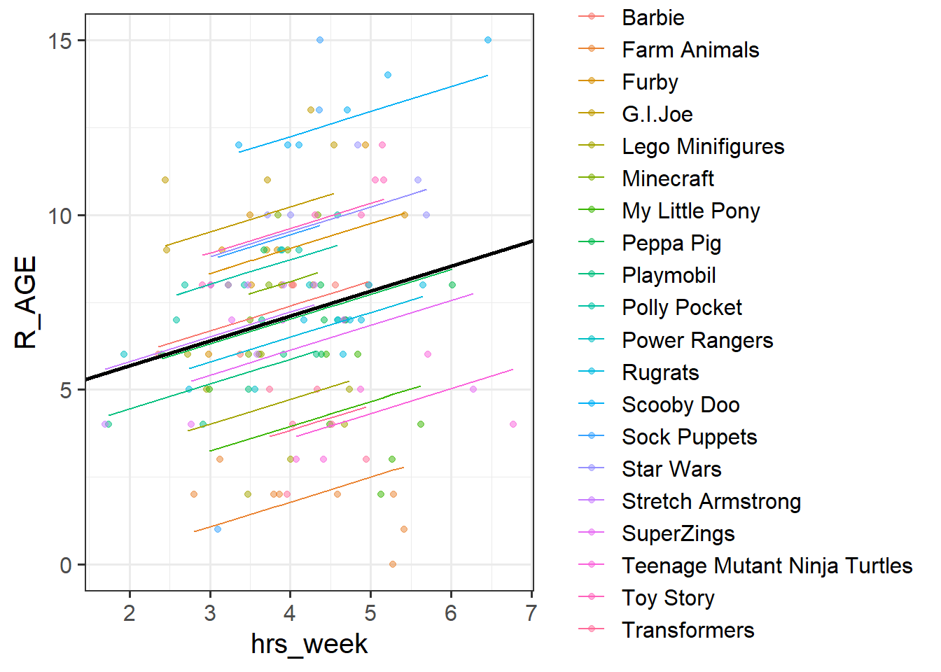
Question 3

From the previous questions you should have a model called ri_mod.

Below is a plot of the fitted values from that model. Rather than having a separate facet for each type of toy as we did above, I have put them all on one plot. The thick black line is the average intercept and slope of the toy-type lines.

Identify the parts of the plot that correspond to A1-4 in the summary output of the model below

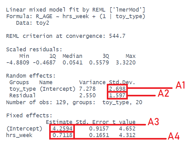
Hints

Choose from these options:

• where the black line cuts the y axis (at x=0)
  
• the slope of the black line
  
• the standard deviation of the distances from all the individual datapoints (toys) to their respective toy-type lines
  
• the standard deviation of the distances from all the toy-type lines to the black line

Solution 3.

• A1 = the standard deviation of the distances from all the toy-type lines to the black line
  
• A2 = the standard deviation of the distances from all the individual datapoints (toys) to their respective toy-type lines
  
• A3 = where the black line cuts the y axis
  
• A4 = the slope of the black line

Optional Extra

Below is the model equation for the ri_mod model.

Identify the part of the equation that represents each of A1-4.

\[\begin{align} \text{For Toy }j\text{ of Type }i & \\ \text{Level 1 (Toy):}& \\ \text{R\_AGE}_{ij} &= b_{0i} + b_1 \cdot \text{hrs\_week}_{ij} + \epsilon_{ij} \\ \text{Level 2 (Type):}& \\ b_{0i} &= \gamma_{00} + \zeta_{0i} \\ \text{Where:}& \\ \zeta_{0i} &\sim N(0,\sigma_{0}) \\ \varepsilon &\sim N(0,\sigma_{e}) \\ \end{align}\]

Hints

Choose from:

• \(\sigma_{\varepsilon}\)
  
• \(b_{1}\)
  
• \(\sigma_{0}\)
  
• \(\gamma_{00}\)

Solution 4.

• A1 = \(\sigma_{0}\)
  
• A2 = \(\sigma_{\varepsilon}\)
  
• A3 = \(\gamma_{00}\)
  
• A4 = \(b_{1}\)

Audio Interference in Executive Functioning (Repeated Measures)

This next set are closer to conducting a real study. We have some data and a research question (below). The exercises will walk you through describing the data, then prompt you to think about how we might fit an appropriate model to address the research question, and finally task you with having a go at writing up what you’ve done.

Data: Audio interference in executive functioning

This data is from a simulated study that aims to investigate the following research question:

How do different types of audio interfere with executive functioning, and does this interference differ depending upon whether or not noise-cancelling headphones are used?

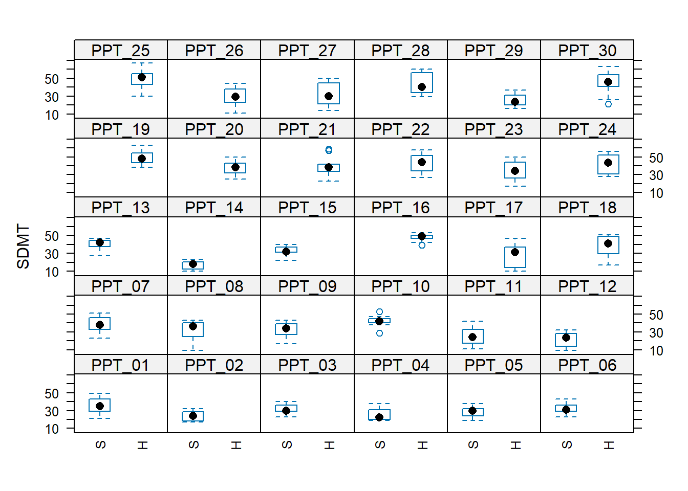
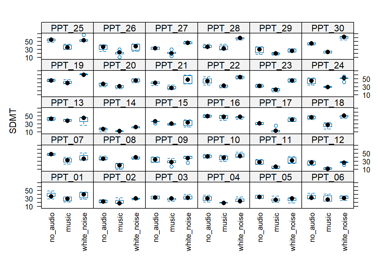
30 healthy volunteers each completed the Symbol Digit Modalities Test (SDMT) - a commonly used test to assess processing speed and motor speed - a total of 15 times. During the tests, participants listened to either no audio (5 tests), white noise (5 tests) or classical music (5 tests). Half the participants listened via active-noise-cancelling headphones, and the other half listened via speakers in the room. Unfortunately, lots of the tests were not administered correctly, and so not every participant has the full 15 trials worth of data.

The data is available at https://uoepsy.github.io/data/lmm_ef_sdmt.csv.

variable	description
PID	Participant ID
audio	Audio heard during the test ('no_audio', 'white_noise','music')
headphones	Whether the participant listened via speakers (S) in the room or via noise cancelling headphones (H)
SDMT	Symbol Digit Modalities Test (SDMT) score

Question 4

How many participants are there in the data?
How many have complete data (15 trials)?
What is the average number of trials that participants completed? What is the minimum?
Does every participant have some data for each type of audio?

Hints

Functions like table() and count() will likely be useful here.

Solution 5.

efdat <- read_csv("https://uoepsy.github.io/data/lmm_ef_sdmt.csv")
head(efdat)

# A tibble: 6 × 4
  PID    audio       headphones  SDMT
  <chr>  <chr>       <chr>      <dbl>
1 PPT_15 no_audio    S             37
2 PPT_22 no_audio    H             55
3 PPT_21 no_audio    H             40
4 PPT_20 no_audio    H             36
5 PPT_20 no_audio    H             30
6 PPT_05 white_noise S             30

Solution 6. For a quick “how many?”, functions like n_distinct() can be handy:

n_distinct(efdat$PID)

[1] 30

Which is essentially the same as asking:

unique(efdat$PID) |> length()

[1] 30

Solution 7. Here are the counts of trials for each participant.

efdat |> 
  count(PID)

# A tibble: 30 × 2
  PID        n
  <chr>  <int>
1 PPT_01    13
2 PPT_02    12
3 PPT_03    10
4 PPT_04    10
5 PPT_05    10
# ℹ 25 more rows

We can pass that to something like summary() to get a quick descriptive of the n column, and so we can see that no participant completed all 15 trials (max is 14). Everyone completed at least 10, and the median was 12.

efdat |> 
  count(PID) |>
  summary()

     PID                  n     
 Length:30          Min.   :10  
 Class :character   1st Qu.:11  
 Mode  :character   Median :12  
                    Mean   :12  
                    3rd Qu.:13  
                    Max.   :14  

We could also do this easily with things like:

table(efdat$PID) |> median()

[1] 12

Solution 8. For this kind of thing I would typically default to using table() for smaller datasets, to see how many datapoints are in each combination of PID and audio:

table(efdat$PID, efdat$audio)

        
         music no_audio white_noise
  PPT_01     4        5           4
  PPT_02     5        4           3
  PPT_03     3        2           5
  PPT_04     3        4           3
  PPT_05     5        2           3
  PPT_06     4        4           5
  PPT_07     4        3           4
  PPT_08     4        4           5
  PPT_09     5        4           5
  PPT_10     4        5           4
  PPT_11     4        4           4
  PPT_12     4        5           5
  PPT_13     4        4           3
  PPT_14     3        5           4
  PPT_15     4        5           4
  PPT_16     4        4           3
  PPT_17     5        4           5
  PPT_18     5        3           3
  PPT_19     3        5           3
  PPT_20     4        4           5
  PPT_21     3        5           4
  PPT_22     4        4           3
  PPT_23     3        3           4
  PPT_24     4        5           5
  PPT_25     4        4           5
  PPT_26     5        4           5
  PPT_27     5        2           4
  PPT_28     4        4           4
  PPT_29     4        4           4
  PPT_30     2        5           3

From the above, we can see that everyone has data from \(\geq 2\) trials for a given audio type.

table(efdat$PID, efdat$audio) |> min()

[1] 2

a tidyverse way:

When tables get too big, we can do the same thing with count(), but we need to make sure that we are working with factors, in order to summarise all possible combinations of groups (even empty ones)

efdat |> 
  mutate(PID = factor(PID),
         audio = factor(audio)) |>
  # the .drop=FALSE means "keep empty groups"
  count(PID,audio,.drop=FALSE) |> 
  summary()

      PID             audio          n    
 PPT_01 : 3   music      :30   Min.   :2  
 PPT_02 : 3   no_audio   :30   1st Qu.:4  
 PPT_03 : 3   white_noise:30   Median :4  
 PPT_04 : 3                    Mean   :4  
 PPT_05 : 3                    3rd Qu.:5  
 PPT_06 : 3                    Max.   :5  
 (Other):72                               

There are plenty of other ways (e.g., you could use combinations of group_by(), summarise()), so just pick one that makes sense to you.

Question 5

How do different types of audio interfere with executive functioning, and does this interference differ depending upon whether or not noise-cancelling headphones are used?

Consider the following questions about the study:

• What is our outcome of interest?
  
• What variables are we seeking to investigate in terms of their impact on the outcome?
  
• What are the units of observations?
  
• Are the observations clustered/grouped? In what way?
  
• What varies within these clusters?
  
• What varies between these clusters?

Solution 9.

• What is our outcome of interest?
  • SDMT scores
    
• What variables are we seeking to investigate in terms of their impact on the outcome?
  • audio type and the interaction audio type \(\times\) wearing headphones
• What are the units of observations?
  • individual trials
    
• What are the groups/clusters?
  • participants
    
• What varies within these clusters?
  • the type of audio
    
• What varies between these clusters?
  • whether they listen via headphones or speakers

Question 6

Make factors and set the reference levels of the audio and headphones variables to “no audio” and “speakers” respectively.

Hints

Can’t remember about setting factors and reference levels? Check back to USMR!

Solution 10.

efdat <- efdat |>
  mutate(
    audio = fct_relevel(factor(audio), "no_audio"),
    headphones = fct_relevel(factor(headphones), "S")
  )

Question 7

Fit a multilevel model to address the aims of the study (copied below)

How do different types of audio interfere with executive functioning, and does this interference differ depending upon whether or not noise-cancelling headphones are used?

Specifying the model may feel like a lot, but try splitting it into three parts:

\[ \text{lmer(}\overbrace{\text{outcome }\sim\text{ fixed effects}}^1\, + \, (1 + \underbrace{\text{slopes}}_3\, |\, \overbrace{\text{grouping structure}}^2 ) \]

1. Just like the lm()s we have used in the past, think about what we want to test. This should provide the outcome and the structure of our fixed effects.
   
2. Think about how the observations are clustered/grouped. This should tell us how to specify the grouping structure in the random effects.
   
3. Think about which slopes (i.e. which terms in our fixed effects) could feasibly vary between the clusters. This provides you with what to put in as random slopes.

Hints

Make sure to read about multilevel modesl and how to fit them in Chapter 2: MLM #multilevel-models-in-r.

Solution 11. The question
    “How do different types of audio interfere with executive functioning” means we are interested in the effects of audio type (audio) on executive functioning (SDMT scores), so we will want:

lmer(SDMT ~ audio ...

However, the research aim also asks
    “… and does this interference differ depending upon whether or not noise-cancelling headphones are used?”
which suggests that we are interested in the interaction SDMT ~ audio * headphones

lmer(SDMT ~ audio * headphones + ...   

Solution 12. There are lots of ways that our data is grouped.
We have:

• 3 different groups of audio type (no_audio, white_noise, music)
• 2 groups of listening condition (S, H)
• 30 groups of participants (“PPT_01”, “PPT_02”, “PPT_03”, …)

The effects of audio type and headphones are both things we actually want to test - these variables are in our fixed effects. The levels of audio and headphones are not just a random sample from a wider population of levels - they’re a specific set of things we want to compare SDMT scores between.

Compare this with the participants - we don’t care about if there is a difference in SDMT scores between e.g., “PPT_03” and “PPT_28”. The participants themselves are just a sample of people that we have taken from a wider population. This makes thinking of “by-participant random effects” a sensible approach - we model differences between participants as a normal distribution of deviations around some average:

lmer(SDMT ~ audio * headphones + (1 + ... | PID)  

The minimum that we can include is the random intercept. What (1|PID) specifies is that “participants vary in their SDMT scores”. This makes sense - we would expect some participants to have higher executive functioning (and so will tend to score high on the SDMT), and others to have lower functioning (and so tend to score lower).

Solution 13. We can also include a random by-participant effect of audio.
audio|PID specifies that the effect of audio type on SDMT varies by participant. This seems feasible - music might be very distracting (and interfere a lot with the test) for some participants, but have a negligible effect for others.

lmer(SDMT ~ audio * headphones + 
              (1 + audio | PID), data = efdat)

Why can’t we have (headphones|PID)?

Why can we fit (1 + audio | PID) but not (1 + headphones | PID), or both (1 + audio + headphones | PID) or (1 + audio * headphones | PID)?

Remember that y ~ ... + (x | g) is saying “the slope of y~x varies by g”.
Such a sentence only makes sense if each “the slope of y~x” is defined for every (or most) groups.

For the headphones predictor, every participant is either in the “S” (speakers) condition or the “H” (headphones) condition.
This means that “the effect of headphones on SDMT” doesn’t exist for any single participant! This means it makes no sense to try and think of the effect as ‘varying by participant’.

Compare this to the audio predictor, for the effect does exist for a single given participant, therefore it is possible to think of it as being different for different participants (e.g. PPT_30’s performance improves with white noise, but PPT_16’s performance does not).

The plots below may help to cement this idea:

Question 8

We now have a model, but we don’t have any p-values or confidence intervals or anything - i.e. we have no inferential criteria on which to draw conclusions. There are a whole load of different methods available for drawing inferences from multilevel models, which means it can be a bit of a never-ending rabbit hole. For now, we’ll just use the ‘quick and easy’ approach provided by the lmerTest package seen in the lectures.

Using the lmerTest package, re-fit your model, and you should now get some p-values!

Hints

If you use library(lmerTest) to load the package, then every single model you fit will show p-values calculated with the Satterthwaite method.
Personally, I would rather this is not the case, so I often opt to fit specific models with these p-values without ever loading the package:
modp <- lmerTest::lmer(y ~ 1 + x + ....

optional: a model comparison

If we want to go down the model comparison route, we just need to isolate the relevant part(s) of the model that we are interested in.

Remember, model comparison is sometimes a useful way of testing a set of coefficients. For instance, in this example the interaction involves estimating two terms: audiomusic:headphonesH and audiowhite_noise:headphonesH.

To test the interaction as a whole, we can create a model without the interaction, and then compare it. The SATmodcomp() function from the pbkrtest package provides a way of conducting an F test with the same Satterthwaite method of approximating the degrees of freedom:

sdmt_mod <- lmer(SDMT ~ audio * headphones + 
              (1 + audio | PID), data = efdat)
sdmt_res <- lmer(SDMT ~ audio + headphones + 
                   (1 + audio | PID), data = efdat)
library(pbkrtest)
SATmodcomp(largeModel = sdmt_mod, smallModel = sdmt_res)

large : SDMT ~ audio * headphones + (1 + audio | PID)
small (restriction matrix) : 
                             
 0 0 0 0 0.8936904 -0.4486841
 0 0 0 0 0.4486841  0.8936904
     statistic    ndf    ddf   p.value    
[1,]    11.051  2.000 26.909 0.0003136 ***
---
Signif. codes:  0 '***' 0.001 '**' 0.01 '*' 0.05 '.' 0.1 ' ' 1

Solution 14.

sdmt_mod <- lmerTest::lmer(SDMT ~ audio * headphones + 
              (1 + audio | PID), data = efdat)

summary(sdmt_mod)

Linear mixed model fit by REML. t-tests use Satterthwaite's method [
lmerModLmerTest]
Formula: SDMT ~ audio * headphones + (1 + audio | PID)
   Data: efdat

REML criterion at convergence: 2376.2

Scaled residuals: 
     Min       1Q   Median       3Q      Max 
-2.34520 -0.62861  0.05762  0.60807  2.21250 

Random effects:
 Groups   Name             Variance Std.Dev. Corr       
 PID      (Intercept)      51.17    7.153               
          audiomusic       13.69    3.700     0.03      
          audiowhite_noise 15.22    3.901    -0.25 -0.16
 Residual                  31.49    5.612               
Number of obs: 360, groups:  PID, 30

Fixed effects:
                             Estimate Std. Error       df t value Pr(>|t|)    
(Intercept)                  33.25799    1.98897 28.22065  16.721 3.54e-16 ***
audiomusic                   -8.01731    1.41149 27.58766  -5.680 4.58e-06 ***
audiowhite_noise             -0.03044    1.44502 26.32588  -0.021 0.983354    
headphonesH                   6.85313    2.81170 28.19226   2.437 0.021355 *  
audiomusic:headphonesH       -3.58748    2.00129 27.94011  -1.793 0.083875 .  
audiowhite_noise:headphonesH  8.02458    2.04498 26.46166   3.924 0.000556 ***
---
Signif. codes:  0 '***' 0.001 '**' 0.01 '*' 0.05 '.' 0.1 ' ' 1

Correlation of Fixed Effects:
            (Intr) audmsc adwht_ hdphnH adms:H
audiomusic  -0.174                            
audiowht_ns -0.352  0.192                     
headphonesH -0.707  0.123  0.249              
admsc:hdphH  0.123 -0.705 -0.135 -0.173       
adwht_ns:hH  0.249 -0.136 -0.707 -0.351  0.191

Question 9

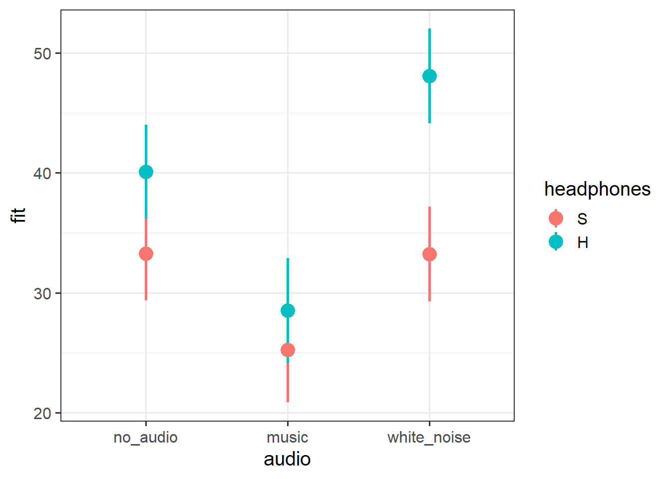
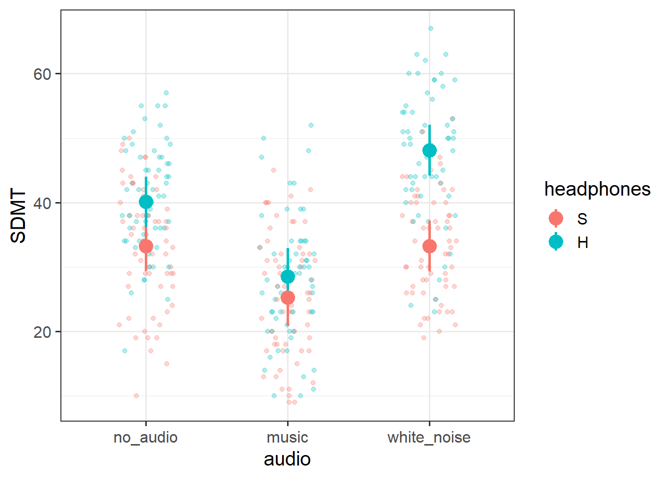
We’ve already seen in the example with the with the different types of toys (above) that we can visualise the fitted values (model predictions). But these were plotting all the cluster-specific values, and what we are really interested in are the estimates of (and uncertainty around) our fixed effects (i.e. estimates for clusters on average)

Using tools like the effects package can provide us with the values of the outcome across levels of a specific fixed predictor (holding other predictors at their mean).

This should get you started:

library(effects)
effect(term = "audio*headphones", mod = sdmt_mod) |>
  as.data.frame()

Hints

You can see the effects package in Chapter 2: MLM #visualising-models. The logic is just the same as it was for USMR, it’s just that the estimated effects are from an lmer() instead of an lm()/glm().

Solution 15.

library(effects)
effect(term = "audio*headphones", mod = sdmt_mod) |>
  as.data.frame() |>
  ggplot(aes(x=audio,y=fit,
             ymin=lower,ymax=upper,
             col=headphones))+
  geom_pointrange(size=1,lwd=1)

Question 10

Now we have some p-values and a plot, try to create a short write-up of the analysis and results.

Hints

Think about the principles that have guided you during write-ups thus far.

The aim in writing a statistical report should be that a reader is able to more or less replicate your analyses without referring to your analysis code. Furthermore, it should be able for a reader to understand and replicate your work even if they use something other than R. This requires detailing all of the steps you took in conducting the analysis, but without simply referring to R code.

• Provide a description of the sample that is used in the analysis, and any steps that you took to get this sample (i.e. data cleaning/removal)
• Describe the model/test and how it addresses the research question. What is the structure of the model, and how did you get to this model? (You don’t need a fancy model equation, you can describe in words!).
• Present (visually and numerically) the key results of the coefficient tests or model comparisons, and explain what these mean in the context of the research question (this could be things like practical significance of the effect size, and the group-level variability in the effects).

Solution 16.

Not a perfect write-up (there’s not really any such thing!).

SDMT scores were modelled using linear mixed effects regression, with fixed effects of audio-type (no audio/white noise/music, treatment coded with no audio as the reference level), audio delivery (speakers vs ANC-headphones, treatment coded with speakers as the reference level) and their interaction. Participant-level random intercepts and random slopes of audio-type were also included. The inclusion of the interaction term between audio-type and audio-delivery was used to address the question of whether the interference of different audio on executive function depends on whether it is heard via noise-cancelling headphones. A model comparison was conducted between the full model and a restricted model that was identical to the full model with the exception that the interaction term was excluded. Models were fitted using the lme4 package in R, and estimated with restricted estimation maximum likelihood (REML). Denominator degrees of freedom for all comparisons and tests were approximated using the Satterthwaite method.

Inclusion of the interaction between headphones and audio-type was found to improve model fit (\(F(2, 26.9) = 11.05, p < .001\)), suggesting that the interference of different types of audio on executive functioning is dependent upon whether the audio is presented through ANC-headphones or through speakers.

Participants not wearing headphones and presented with no audio scored on average 33.26 on the SDMT. For participants without headphones, listening to music via speakers was associated with lower scores compared to no audio (\(b = -8.02, t(27.59)=-5.68, p <0.001\)), but there was no significant difference between white noise and no audio.

With no audio playing, wearing ANC-headphones was associated with higher SDMT scores compared to those wearing no headphones (\(b = 6.85, t(28.19)=2.44, p =0.021\)). The apparent detrimental effect of music on SDMT scores was not significantly different in the headphones condition compared to the no-headphones condition (\(b = -3.59, t(27.94)=-1.79, p =0.084\)). Compared to those listening through speakers, white noise was associated with a greater increase in scores over no audio, when listening via ANC-heaphones (\(b = 8.02, t(26.46)=3.92, p <0.001\)).

There was considerable variability in baseline (i.e. no-audio) SDMT scores across participants (SD = 7.15), with participants showing similar variability in the effects of music (SD = 3.7) and of white-noise (SD = 3.9). A weak negative correlation (-0.25) between participant-level intercepts and effects of white-noise indicated that people who score higher in the no-audio condition tended to be more negatively effect by white-noise. A similar weak negative correlation (-0.16) between music and white-noise effects suggests participants who were more positively affected by one type of audio tended to be more negatively affected by the other.

These results suggest that music appears to interfere with executive functioning (lower SDMT scores) compared to listening to no audio, and this is not dependent upon whether is heard through headphones or speakers. When listening via speakers, white noise was not associated with differences in executive functioning compared to no audio, but this was different for those listening via headphones, in which white noise saw a greater increase in performance. Furthermore, there appear to be benefits for executive functioning from wearing ANC-headphones even when not-listening to audio, perhaps due to the noise cancellation. The pattern of findings are displayed in Figure 1.

Figure 1: Interaction between the type (no audio/white noise/music) and the delivery (speakers/ANC headphones) on executive functioning task (SDMT)

	SDMT
Predictors	Estimates	Statistic	p	df
(Intercept)	33.26	16.72	<0.001	28.22
audio [music]	-8.02	-5.68	<0.001	27.59
audio [white_noise]	-0.03	-0.02	0.983	26.33
headphones [H]	6.85	2.44	0.021	28.19
audio [music] × headphones [H]	-3.59	-1.79	0.084	27.94
audio [white_noise] × headphones [H]	8.02	3.92	0.001	26.46
Random Effects
σ2	31.49
τ00 PID	51.17
τ11 PID.audiomusic	13.69
τ11 PID.audiowhite_noise	15.22
ρ01	0.03
	-0.25
ICC	0.64
N PID	30
Observations	360
Marginal R2 / Conditional R2	0.392 / 0.783

Footnotes

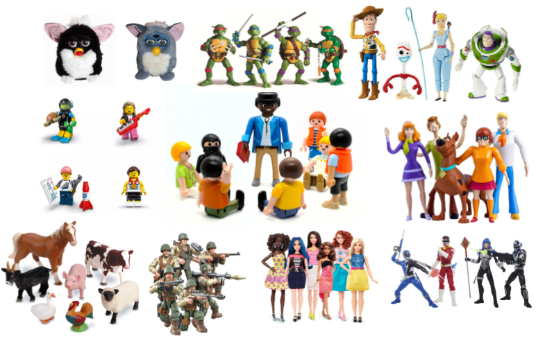
1. Image sources:
   http://tophatsasquatch.com/2012-tmnt-classics-action-figures/
   https://www.dezeen.com/2016/02/01/barbie-dolls-fashionista-collection-mattel-new-body-types/
   https://www.wish.com/product/5da9bc544ab36314cfa7f70c
   https://www.worldwideshoppingmall.co.uk/toys/jumbo-farm-animals.asp
   https://www.overstock.com/Sports-Toys/NJ-Croce-Scooby-Doo-5pc.-Bendable-Figure-Set-with-Scooby-Doo-Shaggy-Daphne-Velma-and-Fred/28534567/product.html
   https://tvtropes.org/pmwiki/pmwiki.php/Toys/Furby
   https://www.fun.com/toy-story-4-figure-4-pack.html
   https://www.johnlewis.com/lego-minifigures-71027-series-20-pack/p5079461