Covariance and correlation

1. Understand when and how to calculate the summary statistics of covariance and correlation, and how to do this in R.
2. Learn what different strengths and directions of correlation look like when visualised as a scatterplot of two quantitative variables.
   
3. Learn how to conduct a test to determine whether a correlation is different from zero.

Recap

In weeks 7-10 of semester 2, we were dealing with a quantitative response variable and a categorical explanatory variables.

Test	Description
One-sample t-test	tests whether the mean of a sample (\(\mu\)) is significantly different from an hypothesised value (\(\mu_0\), typically equal to 0)
Two-samples t-test	tests whether the difference in the means of two samples (\(\mu_1 - \mu_2\)) is significantly different from an hypothesised value (\(\mu_0\), typically equal to 0)
Paired-samples t-test	tests whether the mean of the differences computed from paired samples (\(\mu_d\)) is significantly different from an hypothesised value (\(\mu_0\), typically equal to 0)

Last week, we began working with categorical response variables. We discussed the chi-square goodness-of-fit test and the chi-square test of independence:

Test	Description
\(\chi^2\) goodness-of-fit	tests whether categorical variable conforms with hypothesized proportions
\(\chi^2\) independence	tests whether categorical variable is related to another categorical variable

This week, we will cover associations between two quantitative variables.

Two quantitative variables

Over the past few weeks we’ve looked at different types of variables (outlined above in the recap). Thinking of previous ways we’ve visualised the data (histograms, bar plots). Now we’re focusing on two continuous variables.

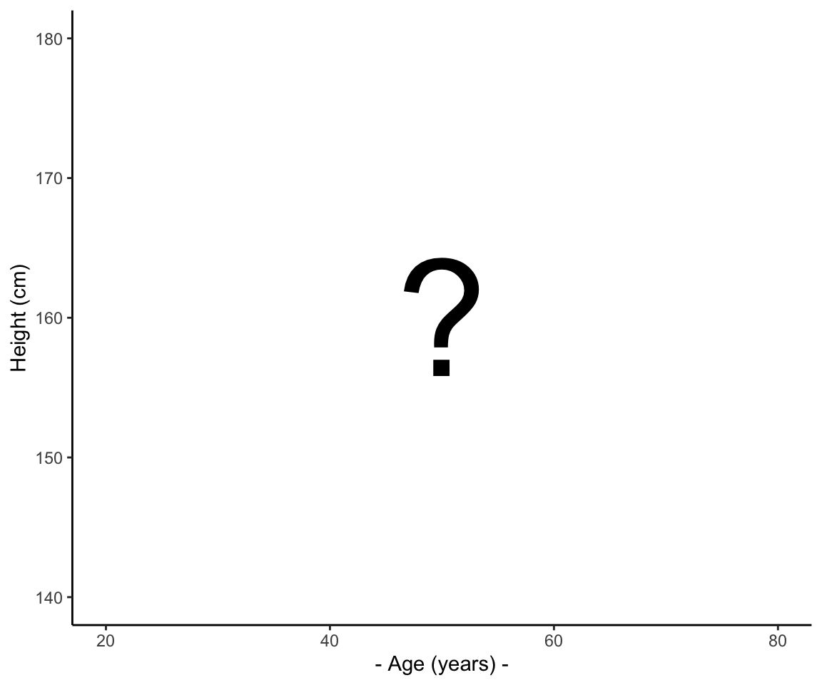
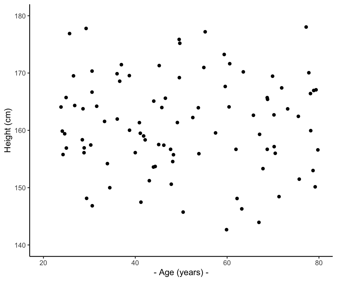
How would you visualise two quantitative variables such as age and height?

Question

How would you most often visualise the relationship between two quantitative variables?

What should we fill this plot with?

Solution

A scatterplot!

If you record two numeric variables \(X\) and \(Y\) for each unit, you can represent each uni as a point on a 2D plane.

Variance vs Covariance

Covariance and variance are two commonly used terms in statistics - they sound similar but they’re quite different! It’s worth looking at both variance and covariance to understand their differences and when to use them.

• Variance: measures how spread out are the data values around the mean.

• Covariance: measures how the values of one variable are associated values in the other variable.

Variance

Variance measures how spread out values are in a given dataset. The variance is the average squared deviation from the mean. The sample variance \(s^2\), it is an unbiased estimator of the population variance.

Unbiased estimator

An estimator of a given parameter is said to be unbiased if its expected value is equal to the true value of the parameter. In other words, an estimator is unbiased if it produces parameter estimates that are, on average, correct.

For example, The sample variance (\(s^2\)) is an unbiased estimator for the population variance (\(\sigma^2\)) as per definition: \[ E(s^2)=\sigma^2 \]

Variance is used when you wish to quantify how spread out values are in a dataset. The higher the variance value, the more spread out they are around the mean.

Formula (sample variance)

The formula to find the variance of a sample (\(s^2\)) is:

\[ s^2 = \frac{\sum (x_i - \overline{x})^2}{n-1} \] where:

• \(\sum\): the sum over all data values
• \(\overline{x}\): the sample mean
• \(x_i\): the \(i\)th observation in the sample
• \(n\): sample size

Variance example

ex1 <- c(1, 2, 3, 4, 5, 5, 12, 14, 20, 13, 
         6, 7, 10, 13, 14, 14, 18, 19, 22, 24) # dataset with 20 values 
var(ex1)

## [1] 48.74737

ex2 <- c(55, 34, 43, 65, 65, 43, 49, 24, 19, 10,
         6, 13, 19, 24, 25, 30, 36, 43, 49, 55) # another dataset of 20 values
var(ex2) 

## [1] 316.45

For the first example dataset, the sample variance is 48.75 and the second dataset has a sample variance of 316.45

As the variance is larger for the second example dataset, this indicates that the values in the second data set are more spread out vs the values in the first example set.

Covariance

Covariance measures how the values in one variable are associated with the values of another variable. That is, what values of one variables are typically observed with other values of another variable.

Covariance is a measure of association between two numeric variable.

• Positive association (positive covariance) indicates that higher values of one variable tend to be observed with higher values of the other variable, or that lower values of one variable tend to be associated with lower values of the other variable.

• Negative association (negative covariance) indicates that higher values of one variable tend to be observed with lower values of the other variable, or that lower values of one variable tend to be associated with higher values of the other variable.

Formula (sample covariance)

\[ \text{Cov}(X,Y) = \frac{\sum (x_i - \overline{x})(y_i - \overline{y})}{n-1} \]

where:

• \(\sum\): is the sum
• \(x_i\): the \(i\)th observation of variable \(X\)
• \(\overline{x}\): sample mean of variable \(X\)
• \(y_i\): the \(i\)th observation of variable \(Y\)
• \(\overline{y}\): sample mean of variable \(Y\)
• \(n\): total number of pairwise observations

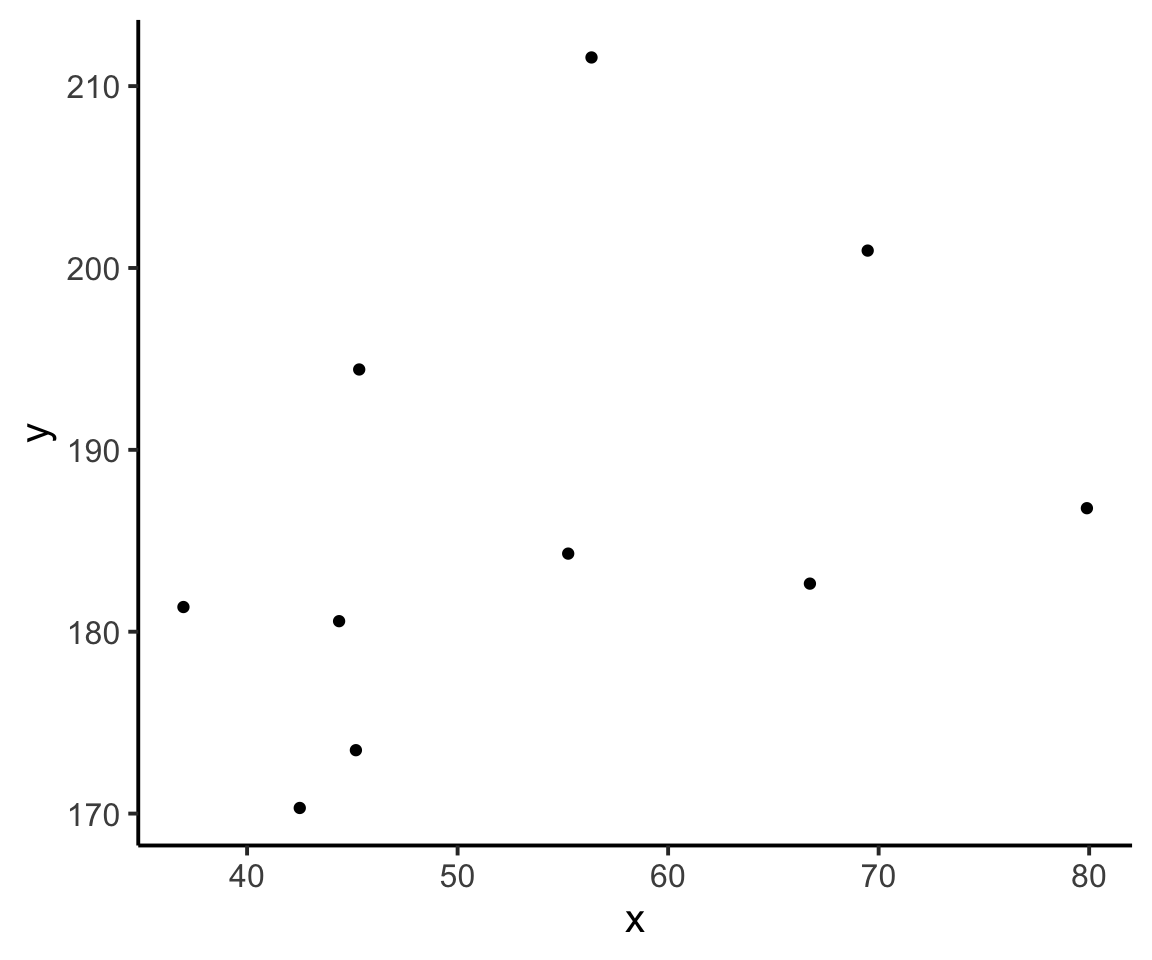
A visual explanation

Consider the following scatterplot:

Now let’s superimpose a vertical dashed line at the mean of \(x\) (\(\bar{x}\)) and a horizontal dashed line at the mean of \(y\) (\(\bar{y}\)):
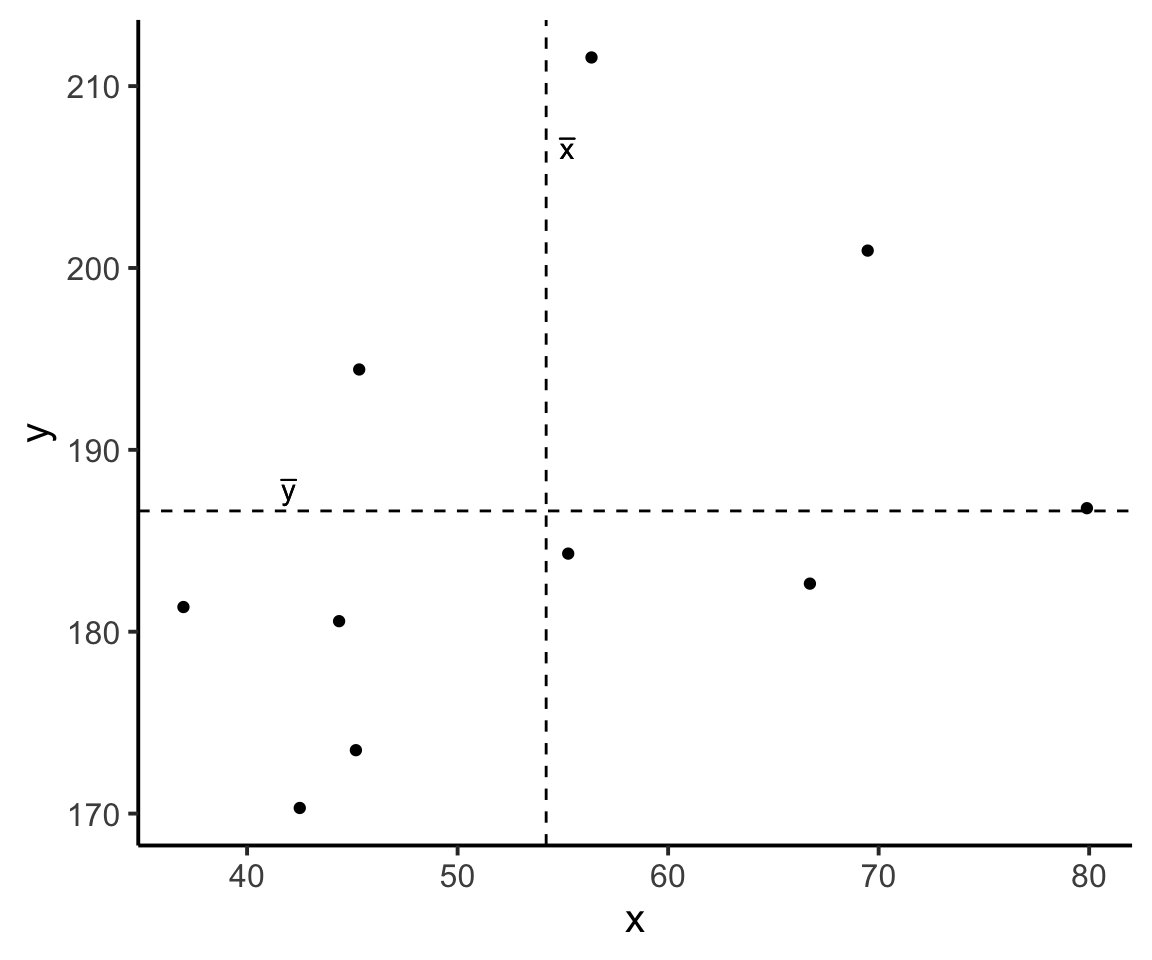
Now let’s pick one of the points, call it \(x_i\), and show \((x_{i}-\bar{x})\) and \((y_{i}-\bar{y})\).

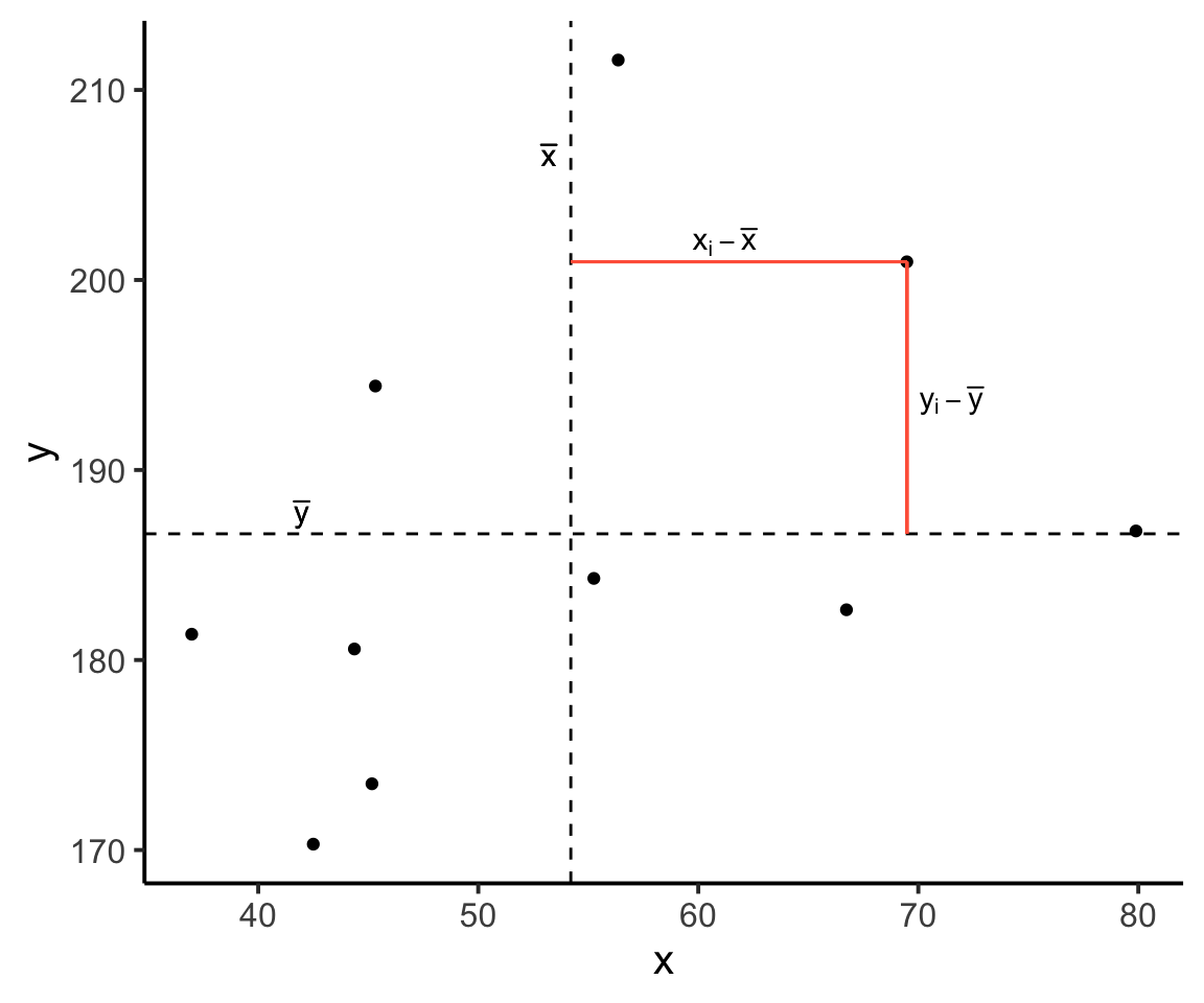Notice that this makes a rectangle.

As \((x_{i}-\bar{x})\) and \((y_{i}-\bar{y})\) are both positive values, their product \((x_{i}-\bar{x})(y_{i}-\bar{y})\) is positive.

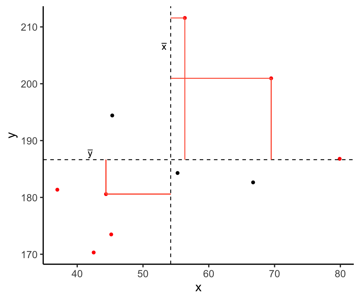
In fact, for all these points in red, the product \((x_{i}-\bar{x})(y_{i}-\bar{y})\) is positive (remember that a negative multiplied by a negative gives a positive):
And for these points in blue, the product \((x_{i}-\bar{x})(y_{i}-\bar{y})\) is negative:

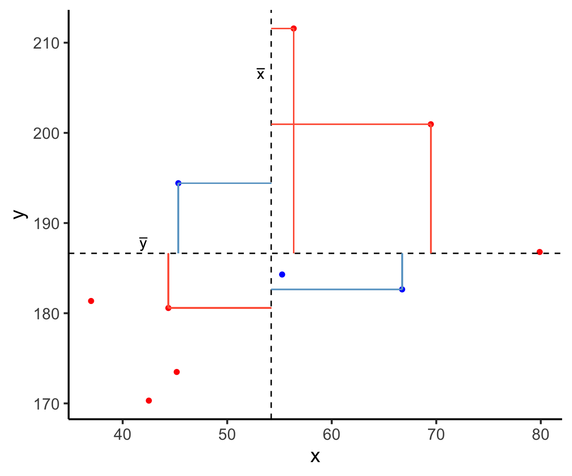
Now take another look at the formula for covariance:

\[\mathrm{Cov}(x,y)=\frac{\sum (x_{i}-\bar{x})(y_{i}-\bar{y})}{n-1}\]

It is the sum of all these products divided by \(n-1\). It is the average of the products!

Covariance example

Suppose we have a an example dataset with 20 values:

example_data <- tibble(ex1, ex2)
example_data

## # A tibble: 20 × 2
##      ex1   ex2
##    <dbl> <dbl>
##  1     1    55
##  2     2    34
##  3     3    43
##  4     4    65
##  5     5    65
##  6     5    43
##  7    12    49
##  8    14    24
##  9    20    19
## 10    13    10
## 11     6     6
## 12     7    13
## 13    10    19
## 14    13    24
## 15    14    25
## 16    14    30
## 17    18    36
## 18    19    43
## 19    22    49
## 20    24    55

Calculating the covariance manually, we’ll first need to calculate the mean score for ex1 and ex2:

example_data <- example_data %>%
  mutate(
    mean_ex1 = mean(ex1),
    mean_ex2 = mean(ex2)
  )

example_data

## # A tibble: 20 × 4
##      ex1   ex2 mean_ex1 mean_ex2
##    <dbl> <dbl>    <dbl>    <dbl>
##  1     1    55     11.3     35.4
##  2     2    34     11.3     35.4
##  3     3    43     11.3     35.4
##  4     4    65     11.3     35.4
##  5     5    65     11.3     35.4
##  6     5    43     11.3     35.4
##  7    12    49     11.3     35.4
##  8    14    24     11.3     35.4
##  9    20    19     11.3     35.4
## 10    13    10     11.3     35.4
## 11     6     6     11.3     35.4
## 12     7    13     11.3     35.4
## 13    10    19     11.3     35.4
## 14    13    24     11.3     35.4
## 15    14    25     11.3     35.4
## 16    14    30     11.3     35.4
## 17    18    36     11.3     35.4
## 18    19    43     11.3     35.4
## 19    22    49     11.3     35.4
## 20    24    55     11.3     35.4

Next, to create three new columns which are:

1. ex1 value - mean of ex1: the \((x_i - \overline{x})\) part
2. ex2 value - mean of ex2: the \((y_i - \overline{y})\) part
3. the product of 1. and 2.: calculating the \((x_i - \overline{x})(y_i - \overline{y})\) part

example_data <- example_data %>%
  mutate(
    xixbar = ex1 - mean_ex1,
    yiybar = ex2 - mean_ex2,
    prod = xixbar * yiybar
  )

example_data

## # A tibble: 20 × 7
##      ex1   ex2 mean_ex1 mean_ex2  xixbar  yiybar    prod
##    <dbl> <dbl>    <dbl>    <dbl>   <dbl>   <dbl>   <dbl>
##  1     1    55     11.3     35.4 -10.3    19.6   -202.  
##  2     2    34     11.3     35.4  -9.3    -1.35    12.6 
##  3     3    43     11.3     35.4  -8.3     7.65   -63.5 
##  4     4    65     11.3     35.4  -7.3    29.6   -216.  
##  5     5    65     11.3     35.4  -6.3    29.6   -187.  
##  6     5    43     11.3     35.4  -6.3     7.65   -48.2 
##  7    12    49     11.3     35.4   0.700  13.6      9.55
##  8    14    24     11.3     35.4   2.7   -11.4    -30.6 
##  9    20    19     11.3     35.4   8.7   -16.4   -142.  
## 10    13    10     11.3     35.4   1.7   -25.4    -43.1 
## 11     6     6     11.3     35.4  -5.3   -29.4    156.  
## 12     7    13     11.3     35.4  -4.3   -22.4     96.1 
## 13    10    19     11.3     35.4  -1.3   -16.4     21.3 
## 14    13    24     11.3     35.4   1.7   -11.4    -19.3 
## 15    14    25     11.3     35.4   2.7   -10.4    -27.9 
## 16    14    30     11.3     35.4   2.7    -5.35   -14.4 
## 17    18    36     11.3     35.4   6.7     0.650    4.35
## 18    19    43     11.3     35.4   7.7     7.65    58.9 
## 19    22    49     11.3     35.4  10.7    13.6    146.  
## 20    24    55     11.3     35.4  12.7    19.6    250.

Next, to sum the products and divide by \(n-1\):

example_data %>%
  summarise(
    prod_sum = sum(prod),
    n = n()
  )

## # A tibble: 1 × 2
##   prod_sum     n
##      <dbl> <int>
## 1    -241.    20

-241.1/(20-1)

## [1] -12.68947

As always, R has a useful function so we don’t have to calculate covariance by hand! We’ll use the cov function to make sure we get the same results.

The function cov takes in two variables x = and y =, in this case we want each example variable in our example_data dataset (ex1 and ex2) as all the other columns and values were made to calculate the covariance formula by hand

cov(example_data$ex1, example_data$ex2)

## [1] -12.68947

As we have a negative covariance value, it means that the values of one variable tend to be observed with values of the opposite sign of the other variable.

You may informally think of a negative covariance value as meaning that the movement in one variable is opposite to the movement of the other variable. For instance:

• if X is moving upwards, Y is moving downwards
• if X is moving downwards, Y is moving upwards

If we have a positive covariance value, the opposite is true: the movement in one variable is the same to the movement of the other variable.

Correlation (\(r\))

Correlation can be thought of as a standardised covariance. It ranges from \(-1\) to \(+1\), on which the distance from zero indicates the strength of the relationship. Similar to covariance, positive/negative values reflect the nature of the relationship.

Correlation coefficient

The correlation coefficient is a standardised number which quantifies the strength and direction of the linear relationship between 2 variables:

• in a population, it is denoted by the Greek letter \(\rho\) (“rho”)
• in a sample, it is denoted by \(r\)

Formula

To calculate \(r\), we use the following formula:

\[ r_{x,y} = \frac{\text{Cov}(x,y)}{s_x s_y} \] This can be expanded to:

\[ r_{x,y} = \frac{\frac{\sum{(x_i - \bar{x})(y_i - \bar{y})}}{n-1}}{\sqrt{\frac{\sum{(x_i - \bar{x})}^2}{n-1}} \sqrt{\frac{\sum{(x_i - \bar{x})}^2}{n-1}}} \]

But don’t fret! This can be rearranged to:

\[ r_{x,y}=\frac{1}{n-1} \sum \left( \frac{x_{i}-\bar{x}}{s_x} \right) \left( \frac{y_{i}-\bar{y}}{s_y} \right) \] This rearranged formula is very similar to the formula for covariance, but the values \((x_i-\overline{x})\) are divided by the standard deviation \((s_x)\), as are the values \((y_i - \overline{y})\) divided by \(s_y\).

In other words, your are multiplying the z-scores of \(X\) and the z-scores of \(Y\)

\[ r_{x,y}=\frac{\sum z_{x_i} z_{y_i}}{n-1} \]

This standardises all the values so that they are expressed as the distance in standard deviations from their means (\(\overline{x}\) and \(\overline{y}\)).

Properties of correlation coefficients

• \(-1 \leq r \leq 1\)
• The sign indicates the direction of association
  • positive correlation (\(r > 0\)) means that the values of one variable tend to be higher when values of the other variable are higher
  • negative correlation (\(r < 0\)) means that values of one variable tend to be lower when values of the other variable are higher
  • no linear correlation (\(r \approx 0\)) means that the higher/lower values of one variable do not tend to occur with higher/lower values of the other variable
• The closer \(r\) is to \(\pm1\), the stronger the linear relationship
• \(r\) has no units and does not depend on the units of measurement
• The correlation between \(x\) and \(y\) is the same as the correlation between \(y\) and \(x\)

Correlation example

Earlier, we calculated that \(\text{Cov}(ex1,ex2) = -12.689\). To calculate the correlation, we simply divide this number by the standard deviations of the two variables.

example_data %>%
  summarise(
    s_ex1 = sd(ex1),
    s_ex2 = sd(ex2)
  )

## # A tibble: 1 × 2
##   s_ex1 s_ex2
##   <dbl> <dbl>
## 1  6.98  17.8

-12.689/(6.981932*17.78904)

## [1] -0.1021643

We can also use the cor() function to calculate our correlation coefficient:

cor(example_data$ex1, example_data$ex2)

## [1] -0.1021681

The numbers are the same (phew). But what does this value mean? As stated above, a negative \(r\) value indicates that as one variable increases, the other decreases. Also note, this value of -0.102 is close to 0, so the relationship is very small.

Testing significance of the correlation coefficient

Now that we’ve seen the formulae for covariance and correlation, as well as their associated functions in R, we can use a statistical test to establish the probability of finding an association this strong by chance alone.

Hypotheses

Null hypothesis

\[ H_0: \rho = 0 \]

I.e. there is no linear association between \(x\) and \(y\) in the population.

Alternative hypothesis

1. (two-sided) \(H_1: \rho \neq 0\) (there is a linear association between \(x\) and \(y\) in the population)
2. (left-tailed) \(H_1: \rho < 0\) (there is a negative linear association between \(x\) and \(y\) in the population)
3. (right-tailed) \(H_1: \rho > 0\) (there is a positive linear association between \(x\) and \(y\) in the population)

Test statistic

Our test statistic is another \(t\) statistic (you can never escape them). The formula for which depends on both the observed correlation (\(r\)) and the sample size (\(n\)):

\[ t = r\sqrt{\frac{n-2}{1-r^2}} \]

where:

• \(r\): correlation coefficient
• \(n\): sample size

p-value

To calculate the p-value for our \(t\)-statistic, it’s the usual format:

1. \(P(t_{n-2} \leq t)\)
2. \(P(t_{n-2} \geq t)\)
3. \(2 \times P(t_{n-2} \geq |t|)\)

where \(t_{n-2}\) denotes a \(t\)-distribution with \(n - 2\) degrees of freedom.

# correlation coefficient
r <- cor(example_data$ex1, example_data$ex2)

# sample size
n <- nrow(example_data)

# t-statistic
t_stat = r * sqrt((n - 2) / (1 - r^2))

#calculate p-value for t, with df = n-2 
2 * (1 - pt(abs(t_stat), df = 18))

## [1] 0.6682039

Unsurprisingly, there is no significant relationship between the two made-up variables.

Alternatively, we can use the cor.test() function in R:

cor.test(x = example_data$ex1, y = example_data$ex2, 
         alternative = "two.sided")

## 
##  Pearson's product-moment correlation
## 
## data:  example_data$ex1 and example_data$ex2
## t = -0.43574, df = 18, p-value = 0.6682
## alternative hypothesis: true correlation is not equal to 0
## 95 percent confidence interval:
##  -0.5211279  0.3564692
## sample estimates:
##        cor 
## -0.1021681

Example: A hypothetical memory test

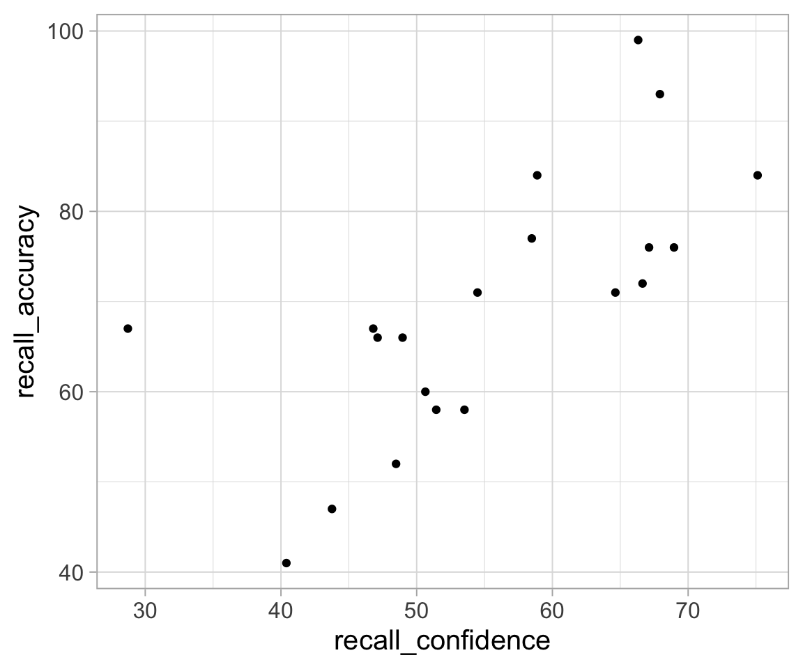
Our data for this example is from a (hypothetical) study on memory. Twenty participants studied passages of text (c500 words long), and were tested a week later. The testing phase presented participants with 100 statements about the text. They had to answer whether each statement was true or false, as well as rate their confidence in each answer (on a sliding scale from 0 to 100). The dataset contains, for each participant, the percentage of items correctly answered, and the average confidence rating. Participants’ ages were also recorded.

Question 1

Read in the data from https://uoepsy.github.io/data/recalldata.csv - it is a .csv file - and look at the dimensions of the data as well as some summary statistics.

Plot the relationship between the percentage of items answered correctly (recall_accuracy) and participants’ average self-rating of confidence in their answers (recall_confidence).

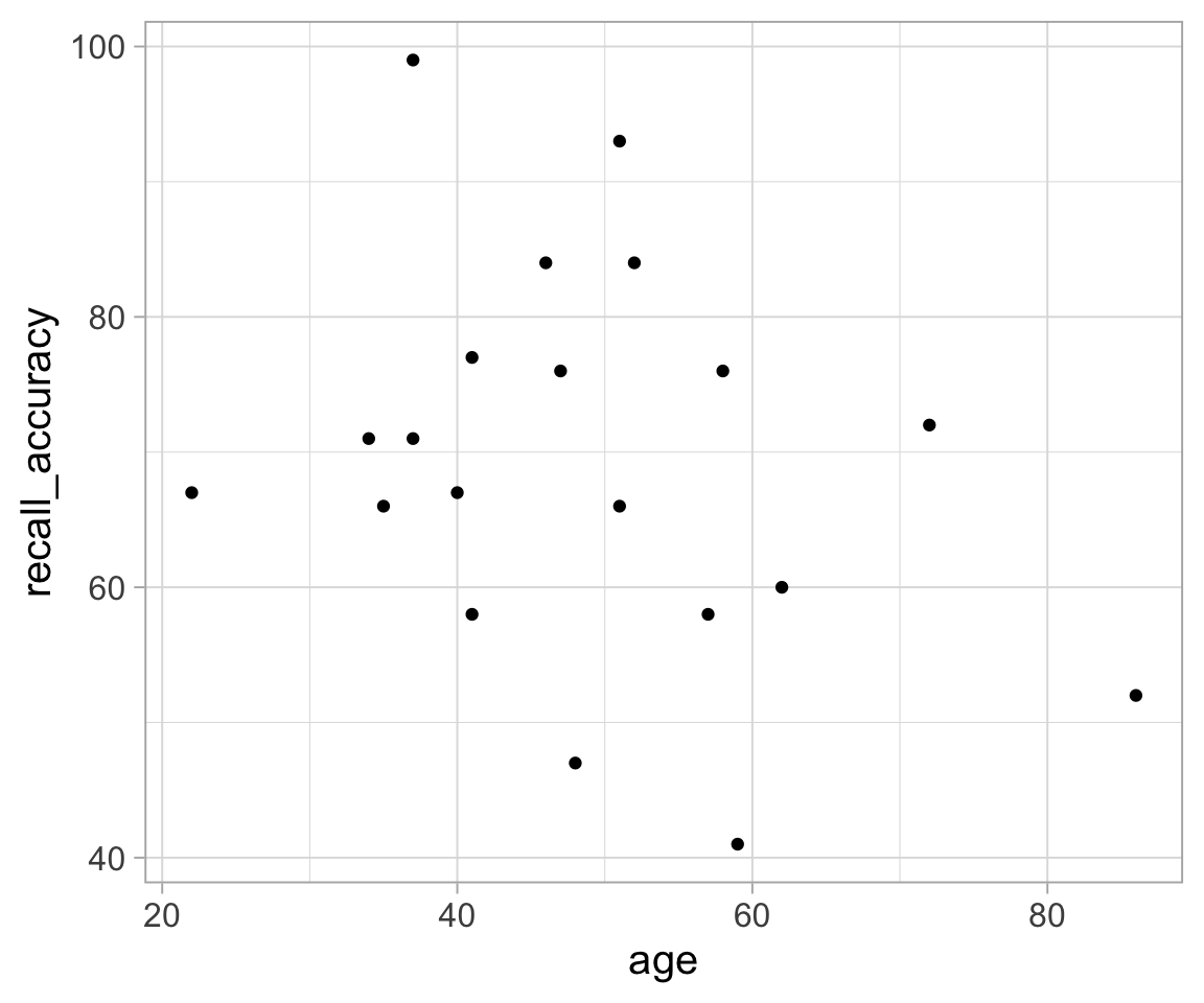
Plot the relationship between recall accuracy and age.

Solution

library(tidyverse)
recalldata <- read_csv("https://uoepsy.github.io/data/recalldata.csv")

dim(recalldata)

## [1] 20  4

summary(recalldata)

##      ppt            recall_accuracy recall_confidence      age       
##  Length:20          Min.   :41.00   Min.   :28.72     Min.   :22.00  
##  Class :character   1st Qu.:59.50   1st Qu.:48.14     1st Qu.:39.25  
##  Mode  :character   Median :69.00   Median :54.00     Median :47.50  
##                     Mean   :69.25   Mean   :55.42     Mean   :48.80  
##                     3rd Qu.:76.25   3rd Qu.:66.40     3rd Qu.:57.25  
##                     Max.   :99.00   Max.   :75.12     Max.   :86.00

ggplot(recalldata, aes(x=recall_confidence, recall_accuracy))+
  geom_point()

ggplot(recalldata, aes(x=age, recall_accuracy))+
  geom_point()

Question 2

We’re going to calculate the covariance between recall accuracy and recall confidence.

Create 2 new columns in the memory recall data, one of which is the mean recall accuracy, and one which is the mean recall confidence.

Remember to assign it using recalldata <- ... otherwise it will just print out the data with the new columns, rather than store it anywhere.

Solution

recalldata <-
  recalldata %>% mutate(
    maccuracy = mean(recall_accuracy),
    mconfidence = mean(recall_confidence)
  )

Question 3

Now create three new columns which are:

1. recall accuracy minus the mean recall accuracy - this is the \((x_i - \bar{x})\) part.
   
2. confidence minus the mean confidence - and this is the \((y_i - \bar{y})\) part.
   
3. the product of i. and ii. - this is calculating \((x_i - \bar{x})\)\((y_i - \bar{y})\).

Solution

recalldata <- 
  recalldata %>% 
    mutate(
      acc_minus_mean_acc = recall_accuracy - maccuracy,
      conf_minus_mean_conf = recall_confidence - mconfidence,
      prod_acc_conf = acc_minus_mean_acc * conf_minus_mean_conf
    )

recalldata

## # A tibble: 20 × 9
##    ppt    recall_accuracy recall_confidence   age maccuracy mconfidence
##    <chr>            <dbl>             <dbl> <dbl>     <dbl>       <dbl>
##  1 ppt_1               72              66.6    72      69.2        55.4
##  2 ppt_2               66              47.1    35      69.2        55.4
##  3 ppt_3               47              43.8    48      69.2        55.4
##  4 ppt_4               84              58.9    52      69.2        55.4
##  5 ppt_5               84              75.1    46      69.2        55.4
##  6 ppt_6               58              53.5    41      69.2        55.4
##  7 ppt_7               52              48.5    86      69.2        55.4
##  8 ppt_8               76              67.1    58      69.2        55.4
##  9 ppt_9               41              40.4    59      69.2        55.4
## 10 ppt_10              67              46.8    22      69.2        55.4
## 11 ppt_11              60              50.6    62      69.2        55.4
## 12 ppt_12              67              28.7    40      69.2        55.4
## 13 ppt_13              76              69.0    47      69.2        55.4
## 14 ppt_14              93              67.9    51      69.2        55.4
## 15 ppt_15              71              54.5    34      69.2        55.4
## 16 ppt_16              71              64.6    37      69.2        55.4
## 17 ppt_17              99              66.3    37      69.2        55.4
## 18 ppt_18              66              49.0    51      69.2        55.4
## 19 ppt_19              77              58.5    41      69.2        55.4
## 20 ppt_20              58              51.4    57      69.2        55.4
## # … with 3 more variables: acc_minus_mean_acc <dbl>,
## #   conf_minus_mean_conf <dbl>, prod_acc_conf <dbl>

Question 4

Finally, sum the products, and divide by \(n-1\)

Solution

recalldata %>%
  summarise(
    prod_sum = sum(prod_acc_conf),
    n = n()
  )

## # A tibble: 1 × 2
##   prod_sum     n
##      <dbl> <int>
## 1    2243.    20

2243.46 / (20-1)

## [1] 118.0768

cov()

Question 5

Check that you get the same results using cov() function.

Hint: cov() can take two variables cov(x = , y = ). Think about how you can use the $ to pull out the variables we are using here.

Solution

It’s the same number!

cov(recalldata$recall_accuracy, recalldata$recall_confidence)

## [1] 118.0768

Question 6

We calculated above that \(\mathrm{Cov}(\texttt{recall_accuracy}, \texttt{recall_confidence})\) = 118.077.

To calculate the correlation, we simply divide this by the standard deviations of the two variables. \(s_{\texttt{recall_accuracy}} \times s_{\texttt{recall_confidence}}\).
Try doing this now.

Solution

recalldata %>% summarise(
  s_ra = sd(recall_accuracy),
  s_rc = sd(recall_confidence)
)

## # A tibble: 1 × 2
##    s_ra  s_rc
##   <dbl> <dbl>
## 1  14.5  11.6

118.08 / (14.527 * 11.622)

## [1] 0.6993902

cor()

Question 7

Just like R has a cov() function for calculating covariance, there is a cor() function for calculating correlation!
They work in a similar way. Try using cor() now and check that we get the same result as above (or near enough, remember that we rounded some numbers above).

Solution

cor(recalldata$recall_accuracy, recalldata$recall_confidence)

## [1] 0.6993654

Correlation matrix

Lots of psychological datasets will have many many related variables. For instance, if a researcher was interested in job satisfaction, they might give a questionnaire to participants, and we would end up with a dataset with lots of variables (one for each question).

We will often want to quickly summarise the relationship between all possible pairs of variables. In the lecture, we saw how to do this using the hetcor() function from the polycor package, giving it a set of variables (or a whole dataset).

You probably won’t have the package polycor yet, so you’ll need to install it first.

Optional: refresher on installing packages

Installing packages

You can install a package either by using install.packages() (for example: install.packages("polycor")), or by choosing the Packages tab in the bottom right window of RStudio, and clicking the install button.

Note: If you run install.packages(), you can do this in the console (the bottom-left window in RStudio).
Remember that the console works like scratch-paper in that nothing you write there is saved.

But we don’t want to save the code which installs packages - if we had it in our RMarkdown document, then every time that you run your code, you will be reinstalling the package.
So running the install.packages() line from a code-chunk in your RMarkdown document is completely fine, just be sure to delete this line of code after you have run it.

Loading packages

Now that we have installed a package, to use it we need to load it first.
This is what we are doing when we use library().

This line you should keep in your code, because it ensures that your code is reproducible. If you don’t include it, then a reader of your code will not know where you got some of the functions from.

Question 9

1. Install the polycor package. You only need to install it once, and you will have access to it forever by calling it via library()
2. Load the polycor package.
   
3. Read in the job satisfaction data from https://uoepsy.github.io/data/jobsat.csv.

Use the function read.csv() rather than read_csv due to a problem with the package polycor.

4. Create a correlation matrix using the function hetcor(), and name it cormat.
   
5. Pull out the correlation matrix using cormat$correlations.

Solution

library(polycor)

jobsat <- read.csv("https://uoepsy.github.io/data/jobsat.csv") 
cormat <- hetcor(jobsat)

cormat$correlations 

##             V1         V2         V3         V4           V5         V6
## V1  1.00000000 0.57616567 0.45024328 0.66141189  0.419666038 0.16564067
## V2  0.57616567 1.00000000 0.46635103 0.45668199  0.387749991 0.23541403
## V3  0.45024328 0.46635103 1.00000000 0.57281285  0.486322359 0.08845336
## V4  0.66141189 0.45668199 0.57281285 1.00000000  0.350897825 0.14580396
## V5  0.41966604 0.38774999 0.48632236 0.35089783  1.000000000 0.06059873
## V6  0.16564067 0.23541403 0.08845336 0.14580396  0.060598731 1.00000000
## V7  0.09906061 0.07566816 0.07147513 0.08959683  0.169030286 0.73800460
## V8  0.10313397 0.09667688 0.10567066 0.14951903  0.027373946 0.66155243
## V9  0.26418653 0.17591843 0.19364178 0.22615489  0.119542129 0.72937420
## V10 0.04566706 0.14640067 0.01933380 0.05912708 -0.003235014 0.45334982
##             V7         V8        V9          V10
## V1  0.09906061 0.10313397 0.2641865  0.045667063
## V2  0.07566816 0.09667688 0.1759184  0.146400667
## V3  0.07147513 0.10567066 0.1936418  0.019333801
## V4  0.08959683 0.14951903 0.2261549  0.059127083
## V5  0.16903029 0.02737395 0.1195421 -0.003235014
## V6  0.73800460 0.66155243 0.7293742  0.453349820
## V7  1.00000000 0.67367531 0.5300598  0.402961387
## V8  0.67367531 1.00000000 0.4490772  0.609851553
## V9  0.53005983 0.44907721 1.0000000  0.540947763
## V10 0.40296139 0.60985155 0.5409478  1.000000000

As it happens, we don’t actually need hetcor() here as we can just use cor() if we like. However, hetcor() can be useful in situations where we want other more complicated types of correlation coefficient to be calculated (see the type argument in in hetcor(x, type = ....)).

cor(jobsat)

It’s a lot of numbers to look at, but each column and each row is a variable, so the left-most column shows the correlations between V1 and each of V1, V2, V3, …, V8.

It is often to difficult to get a good view of the strength and direction of correlations when they are all printed out.
Luckily, we can easily visualise a correlation matrix as a heatmap.

Question 10

1. Install the pheatmap package.
   
2. Load the pheatmap package.
3. visualise your correlation matrix using the function pheatmap().

Solution

library(pheatmap)
pheatmap(cormat$correlations)

Cautions!

Correlation is an invaluable tool for quantifying relationships between variables, but must be used with care.

Below are a few things to be aware of when we talk about correlation.

Caution 1

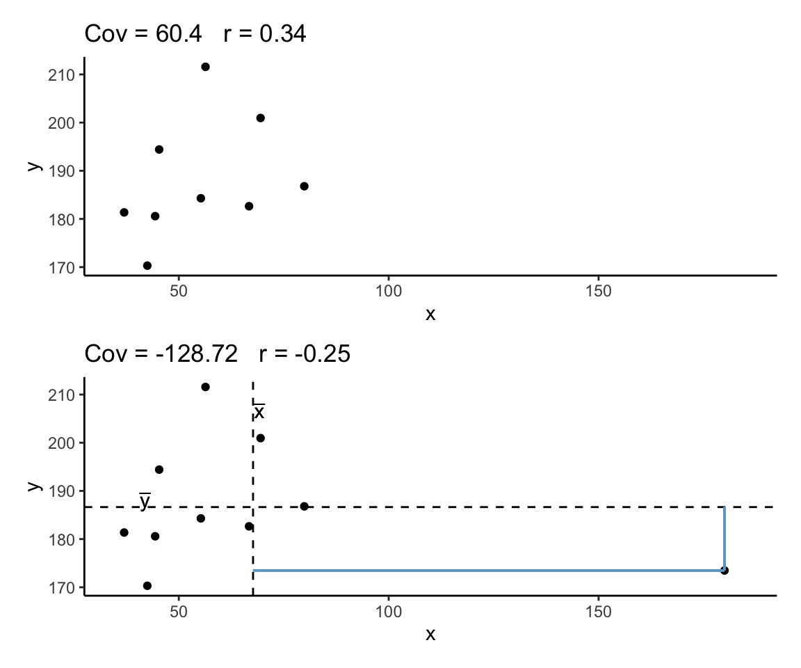
Correlation can be heavily affected by outliers. Always plot your data!

The two plots below only differ with respect to the inclusion of one observation. However, the correlation coefficient for the two sets of observations is markedly different.

Caution 2

Zero correlation (\(r = 0\)) means no linear association. The variables could still be otherwise associated. Always plot your data!

The correlation coefficient in Figure 1 below is negligible, suggesting no linear association. The word “linear” here is crucial - the data are very clearly related.

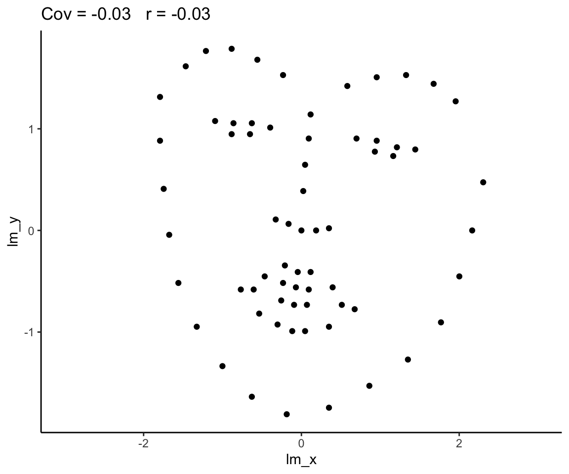
Figure 1: Unrelated data?

Similarly, take look at all the sets of data in Figure 2 below. The summary statistics (means and standard deviations of each variable, and the correlation) are almost identical, but the visualisations suggest that the data are very different from one another.

Figure 2: Datasaurus!

Source: Matejka, J., & Fitzmaurice, G. (2017, May). Same stats, different graphs: generating datasets with varied appearance and identical statistics through simulated annealing. In Proceedings of the 2017 CHI Conference on Human Factors in Computing Systems (pp. 1290-1294).

Caution 3

Correlation does not imply causation!

Figure 3: https://twitter.com/quantitudepod/status/1309135514839248896

You will have likely heard the phrase “correlation does not imply causation”. There is even a whole wikipedia entry devoted to the topic.

Just because you observe an association between x and y, we should not deduce that x causes y

An often cited paper (See Figure 4) which appears to fall foul of this error took a correlation between a country’s chocolate consumption and its number of nobel prize winners to suggest a causal relationship between the two:

Figure 4: Chocolate consumption causes more Nobel Laureates?

“since chocolate consumption has been documented to improve cognitive function, it seems most likely that in a dose-dependent way, chocolate intake provides the abundant fertile ground needed for the sprouting of Nobel laureates”
[Messerli, Franz. Chocolate Consumption, Cognitive Function, and Nobel Laureates. The New England Journal of Medicine 2012; 367:1562-4, (http://www.nejm.org/doi/full/10.1056/NEJMon1211064)]

Example: Sleep and daytime functioning

A researcher is interested in the relationship between hours slept per night and self-rated effects of sleep on daytime functioning. She recruited 50 healthy adults, and collected data on the Total Sleep Time (TST) over the course of a seven day period via sleep-tracking devices.

At the end of the seven day period, participants completed a Daytime Functioning (DTF) questionnaire. This involved participants rating their agreement with ten statements (see Table 1). Agreement was measured on a scale from 1-5.

An overall score of daytime functioning can be calculated by:

1. reversing the scores of items 4, 5 and 6.
   
2. Taking the sum of scores across items.
   
3. Subtracting the summed scores from 50 (the max possible score).

Note: Step 1 is undertaken because those items reflect agreement with positive statements, whereas the other ones are agreement with negative statements. In step 3, subtracting the summed scores from 50 will simply reverse the overall score, meaning that higher scores will indicate better perceived daytime functioning.

The data is available as a .csv at https://uoepsy.github.io/data/sleepdtf.csv.

Table 1: Daytime Functioning Questionnaire

Item	Statement
Item_1	I often felt an inability to concentrate
Item_2	I frequently forgot things
Item_3	I found thinking clearly required a lot of effort
Item_4	I often felt happy
Item_5	I had lots of energy
Item_6	I worked efficiently
Item_7	I often felt irritable
Item_8	I often felt stressed
Item_9	I often felt sleepy
Item_10	I often felt fatigued

Question 11

Read in the data, and calculate the overall daytime functioning score, following the criteria outlined above. Make this a new column in your dataset.

Hint: to reverse items 4, 5 and 6, we we need to make all the scores of 1 become 5, scores of 2 become 4, and so on…

What number satisfies all of these equations?:

• ? - 5 = 1
• ? - 4 = 2
• ? - 3 = 3

Solution

sleepdtf <- read_csv("https://uoepsy.github.io/data/sleepdtf.csv")

# To reverse the items, we can simply do 6 minus the score.   
sleepdtf <- sleepdtf %>%
  mutate(
    item_4_rev = 6 - item_4,
    item_5_rev = 6 - item_5,
    item_6_rev = 6 - item_6
  ) 

# Now to we add them up (be sure to use  the reversed items 4-6)
sleepdtf <- sleepdtf %>%
  mutate(
    dtf = 50-(item_1 + item_2 + item_3 + item_4_rev + item_5_rev + 
          item_6_rev + item_7 + item_8 + item_9 + item_10)
  )

Question 12

Calculate the correlation between the total sleep time (TST) and the overall daytime functioning score.

Solution

cor(sleepdtf$TST, sleepdtf$dtf)

## [1] 0.6694741

Question 13

Conduct a test to establish the probability of observing a correlation this strong in a sample of this size assuming the true correlation to be 0.

Write a sentence or two summarising the results.

Solution

cor.test(sleepdtf$TST, sleepdtf$dtf)

## 
##  Pearson's product-moment correlation
## 
## data:  sleepdtf$TST and sleepdtf$dtf
## t = 6.244, df = 48, p-value = 1.062e-07
## alternative hypothesis: true correlation is not equal to 0
## 95 percent confidence interval:
##  0.4807039 0.7989417
## sample estimates:
##       cor 
## 0.6694741

There was a strong positive correlation between total sleep time and self-reported daytime functioning score (\(r\) = 0.67, \(t(48)\) = 6.24, \(p < .001\)) in the current sample. As total sleep time increased, levels of self-reported daytime functioning increased.

Question 14

Create a correlation matrix of the items in the daytime functioning questionnaire.

You will first need to select the relevant columns.

Solution

To select the relevant columns, there are loads of different methods we can use.
We could do this:

sleepdtf %>% 
  select(item_1, item_2, item_3, item_4, item_5, 
         item_6, item_7, item_8, item_9, item_10)

Or, shorthand, because we know the columns are in order, we can use the following to select everything between item_1 and item_10.

sleepdtf %>% 
  select(item_1:item_10)

Or, yet another option (this one was in the lecture):

sleepdtf[, 2:11]

This will keep all columns from the 2nd column (item_1) to the 11th (item_10).

Refresher

You may remember that there are always lots of ways to do the same thing in R. You may be more comfortable using functions like select(), and filter(), but don’t forget that there are other ways, such as the use of square brackets [], known as ‘indexing’. These can come in pretty handy, so it’s good to have them in your toolbox.

When you index a dataset, you can specify the rows that you want, and the columns that you want mydata[rows, columns].
So we can use:

mydata[1, 4:5]

To give us the first row, and the 4th and 5th columns.

To refresh more of this stuff, it’s worth going back over the very first lab

To make the correlation matrix, we just pass any of these to the hetcor() function from the polycor package!

dtfmatrix <-
  sleepdtf %>% 
  select(item_1:item_10) %>% 
  as.data.frame() %>%
  hetcor()

dtfmatrix$correlations

##              item_1      item_2      item_3      item_4      item_5      item_6
## item_1   1.00000000  0.50837225  0.51273325 -0.17906864 -0.32984013 -0.39313039
## item_2   0.50837225  1.00000000  0.57154789 -0.30744044 -0.13965721 -0.35124536
## item_3   0.51273325  0.57154789  1.00000000 -0.39219980 -0.30066501 -0.23839021
## item_4  -0.17906864 -0.30744044 -0.39219980  1.00000000  0.36480619  0.50052423
## item_5  -0.32984013 -0.13965721 -0.30066501  0.36480619  1.00000000  0.65529215
## item_6  -0.39313039 -0.35124536 -0.23839021  0.50052423  0.65529215  1.00000000
## item_7  -0.03418298  0.08137302  0.32205759 -0.31475066 -0.04393422  0.16140594
## item_8   0.16769150  0.09286012  0.26489465  0.01710394 -0.29071246  0.21594804
## item_9  -0.07923614  0.20620347  0.12972494 -0.14023641  0.04159642  0.30095059
## item_10  0.01083201  0.05563115  0.07139345 -0.35815869 -0.15796053 -0.05114681
##              item_7      item_8      item_9     item_10
## item_1  -0.03418298  0.16769150 -0.07923614  0.01083201
## item_2   0.08137302  0.09286012  0.20620347  0.05563115
## item_3   0.32205759  0.26489465  0.12972494  0.07139345
## item_4  -0.31475066  0.01710394 -0.14023641 -0.35815869
## item_5  -0.04393422 -0.29071246  0.04159642 -0.15796053
## item_6   0.16140594  0.21594804  0.30095059 -0.05114681
## item_7   1.00000000  0.33877450  0.18381414  0.12327218
## item_8   0.33877450  1.00000000  0.32074787  0.09695102
## item_9   0.18381414  0.32074787  1.00000000  0.25787200
## item_10  0.12327218  0.09695102  0.25787200  1.00000000

Question 15

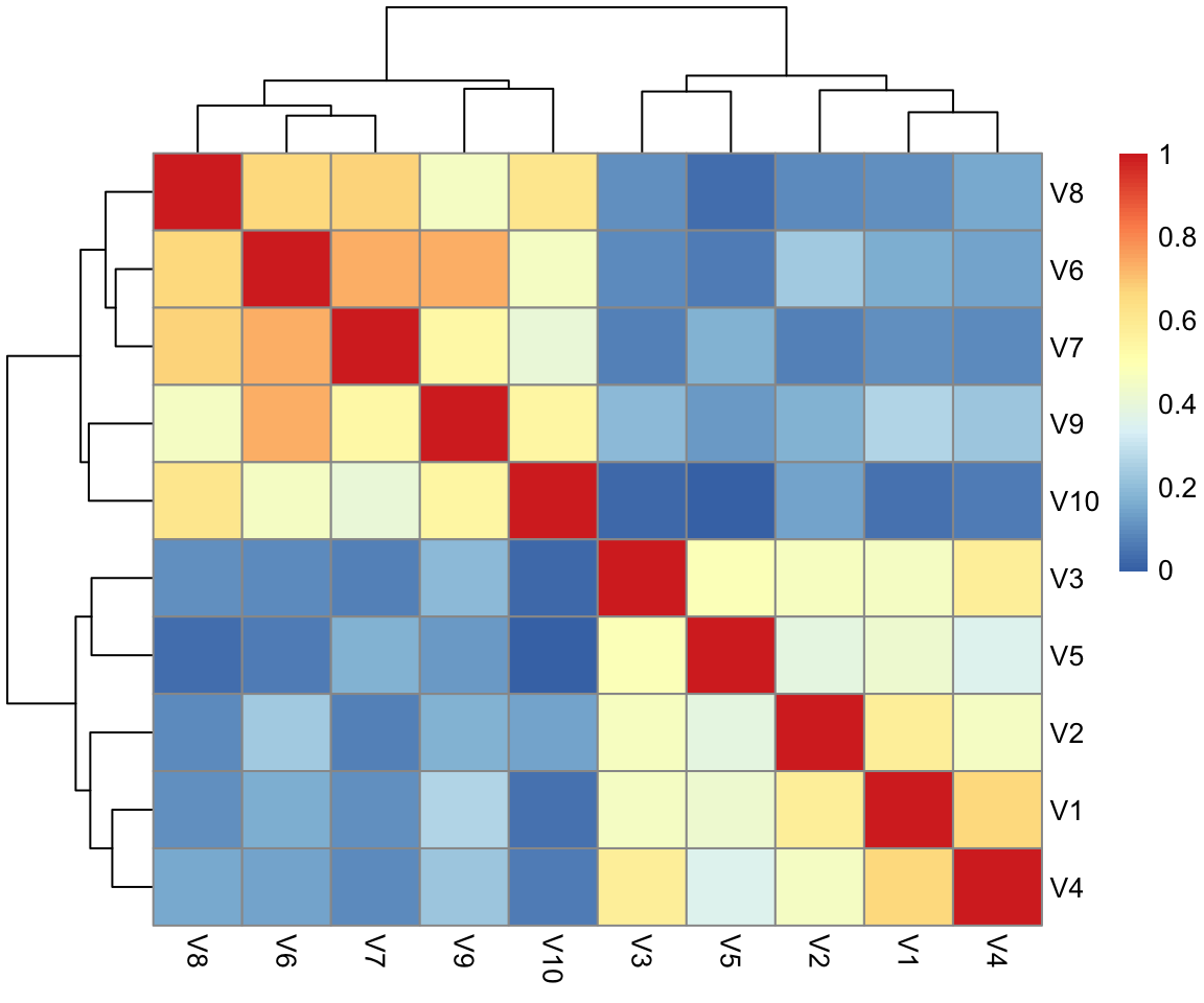
Visualise your correlation matrix using pheatmap() from the pheatmap package.

Solution

pheatmap(dtfmatrix$correlations)

Question 16

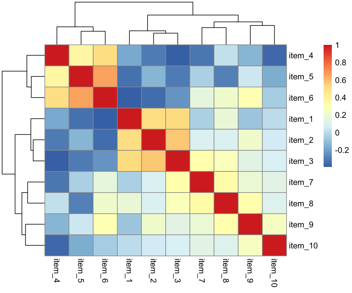
Spend a bit of time thinking about what this correlation matrix shows you, and read the item statements again (Table 1).

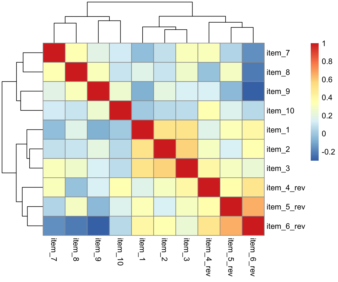
Try creating and visualising a new correlation matrix using the reversed items 4, 5, and 6. What do you expect to be different?

Solution

Items 4, 5, and 6 are all positively correlated with one another, and negatively correlated with Items 1, 2, and 3.

This makes sense, because Items 4, 5, and 6 are all the positive statements, so someone who agrees with those is likely to disagree with the more negative statements.

Furthermore, Items 1, 2, and 3 all seem more strongly correlated with one another than with Items 7, 8, 9 and 10. Are there any differences between these items? It sort of looks like Items 1-3 are all about how well people functioned, whereas 7-10 is about how they felt. This could flag up interesting avenues for future research.

If we change to using the reversed Items 4-6, the direction (but not the strength) of the correlations with these items will change:

# not the most elegant way to do this, but can see clearly what it's doing:
dtfmatrix2 <-
  sleepdtf %>% 
  select(item_1, item_2, item_3, item_4_rev, item_5_rev, 
         item_6_rev, item_7, item_8, item_9, item_10) %>%
  as.data.frame() %>%
  hetcor()

dtfmatrix2$correlations

##                 item_1     item_2     item_3  item_4_rev  item_5_rev
## item_1      1.00000000 0.50837225 0.51273325  0.17906864  0.32984013
## item_2      0.50837225 1.00000000 0.57154789  0.30744044  0.13965721
## item_3      0.51273325 0.57154789 1.00000000  0.39219980  0.30066501
## item_4_rev  0.17906864 0.30744044 0.39219980  1.00000000  0.36480619
## item_5_rev  0.32984013 0.13965721 0.30066501  0.36480619  1.00000000
## item_6_rev  0.39313039 0.35124536 0.23839021  0.50052423  0.65529215
## item_7     -0.03418298 0.08137302 0.32205759  0.31475066  0.04393422
## item_8      0.16769150 0.09286012 0.26489465 -0.01710394  0.29071246
## item_9     -0.07923614 0.20620347 0.12972494  0.14023641 -0.04159642
## item_10     0.01083201 0.05563115 0.07139345  0.35815869  0.15796053
##             item_6_rev      item_7      item_8      item_9    item_10
## item_1      0.39313039 -0.03418298  0.16769150 -0.07923614 0.01083201
## item_2      0.35124536  0.08137302  0.09286012  0.20620347 0.05563115
## item_3      0.23839021  0.32205759  0.26489465  0.12972494 0.07139345
## item_4_rev  0.50052423  0.31475066 -0.01710394  0.14023641 0.35815869
## item_5_rev  0.65529215  0.04393422  0.29071246 -0.04159642 0.15796053
## item_6_rev  1.00000000 -0.16140594 -0.21594804 -0.30095059 0.05114681
## item_7     -0.16140594  1.00000000  0.33877450  0.18381414 0.12327218
## item_8     -0.21594804  0.33877450  1.00000000  0.32074787 0.09695102
## item_9     -0.30095059  0.18381414  0.32074787  1.00000000 0.25787200
## item_10     0.05114681  0.12327218  0.09695102  0.25787200 1.00000000

pheatmap(dtfmatrix2$correlations)

Question 17

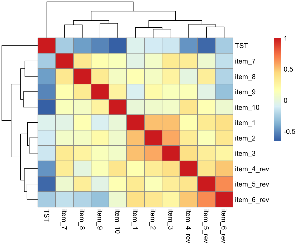
What items on the daytime functioning questionnaire correlate most strongly with the Total Sleep Time (TST)?

Solution

# not the most elegant way to do this, but can see clearly what it's doing:
dtfmatrix3 <-
  sleepdtf %>% 
  select(TST, item_1, item_2, item_3, item_4_rev, item_5_rev, 
         item_6_rev, item_7, item_8, item_9, item_10) %>%
  as.data.frame() %>%
  hetcor()

dtfmatrix3$correlations

##                    TST      item_1      item_2      item_3  item_4_rev
## TST         1.00000000 -0.07080376 -0.12528118 -0.13605652 -0.46651248
## item_1     -0.07080376  1.00000000  0.50837225  0.51273325  0.17906864
## item_2     -0.12528118  0.50837225  1.00000000  0.57154789  0.30744044
## item_3     -0.13605652  0.51273325  0.57154789  1.00000000  0.39219980
## item_4_rev -0.46651248  0.17906864  0.30744044  0.39219980  1.00000000
## item_5_rev -0.61841026  0.32984013  0.13965721  0.30066501  0.36480619
## item_6_rev -0.26036691  0.39313039  0.35124536  0.23839021  0.50052423
## item_7     -0.25544751 -0.03418298  0.08137302  0.32205759  0.31475066
## item_8     -0.43850367  0.16769150  0.09286012  0.26489465 -0.01710394
## item_9     -0.52079536 -0.07923614  0.20620347  0.12972494  0.14023641
## item_10    -0.65895381  0.01083201  0.05563115  0.07139345  0.35815869
##             item_5_rev  item_6_rev      item_7      item_8      item_9
## TST        -0.61841026 -0.26036691 -0.25544751 -0.43850367 -0.52079536
## item_1      0.32984013  0.39313039 -0.03418298  0.16769150 -0.07923614
## item_2      0.13965721  0.35124536  0.08137302  0.09286012  0.20620347
## item_3      0.30066501  0.23839021  0.32205759  0.26489465  0.12972494
## item_4_rev  0.36480619  0.50052423  0.31475066 -0.01710394  0.14023641
## item_5_rev  1.00000000  0.65529215  0.04393422  0.29071246 -0.04159642
## item_6_rev  0.65529215  1.00000000 -0.16140594 -0.21594804 -0.30095059
## item_7      0.04393422 -0.16140594  1.00000000  0.33877450  0.18381414
## item_8      0.29071246 -0.21594804  0.33877450  1.00000000  0.32074787
## item_9     -0.04159642 -0.30095059  0.18381414  0.32074787  1.00000000
## item_10     0.15796053  0.05114681  0.12327218  0.09695102  0.25787200
##                item_10
## TST        -0.65895381
## item_1      0.01083201
## item_2      0.05563115
## item_3      0.07139345
## item_4_rev  0.35815869
## item_5_rev  0.15796053
## item_6_rev  0.05114681
## item_7      0.12327218
## item_8      0.09695102
## item_9      0.25787200
## item_10     1.00000000

pheatmap(dtfmatrix3$correlations)

Question 18

Open-ended: Think about this study in terms of causation.

Claim: Less sleep causes poorer daytime functioning.

Why might it be inappropriate to make the claim above based on these data alone? Think about what sort of study could provide stronger evidence for such a claim.

Things to think about:

• comparison groups.
  
• random allocation.
  
• measures of daytime functioning.
  
• measures of sleep time.
  
• other (unmeasured) explanatory variables.

Glossary

• Variance. A measure of how spread out values are in a data set.
• Covariance. A measure of how changes in one variable area associated with changes in a second variable.
  
• Linear relationship. An equation, when graphed, gives you a straight line - a straight line relationship between two variables. Also known as a linear association.
• Correlation. Measures the linear relationship between two variables \(x\) and \(y\). It has a value between \(-1\) and \(1\).