Independent samples t-test

1. Understand when to use an independent sample \(t\)-test
2. Understand the null hypothesis for an independent sample \(t\)-test
3. Understand how to calculate the test statistic
4. Know how to conduct the test in R
5. Understand the assumptions for \(t\)-tests

Recap: Testing One Mean

Last week you explored how to draw conclusions about a population mean on the basis of the observed sample t-statistic. In particular, given a random sample of size \(n\) from a population, you tested if the population mean was equal to some hypothesized value.

Let the observed sample mean be \(\bar{x}\). Given that the observed sample mean is \(\bar{x}\), we test whether it is plausible that the population mean \(\mu\) could be equal to some hypothesised value \(\mu_0\) (for example 0).

This is done by comparing the observed \(t\)-statistic

\[ t_{obs} = \frac{\bar{x} - \mu_0}{\frac{s}{\sqrt{n}}} \]

with the appropriate critical value from a t distribution with df degrees of freedom.

For an \(\alpha = 0.05\), if the alternative hypothesis \(H_1\) is one-sided we have two cases:

• \(H_1 : \mu > \mu_0\), which has one critical value qt(p = 0.95, df = n - 1)
• \(H_1 : \mu < \mu_0\), which has one critical value qt(p = 0.05, df = n - 1)

If the alternative hypothesis \(H_1\) is two-sided:

• \(H_1 : \mu \neq \mu_0\), we have two critical values qt(p = c(0.025, 0.975), df = n - 1)

We reject the null hypothesis if the observed \(t\)-statistic is as extreme or more extreme than the critical value. Remember, more extreme is calculated in the direction specified by the alternative hypothesis!

The above procedure applies when testing a single parameter (a proportion or a mean) from a single population.

Today you will explore and apply inference procedures for comparing parameters between two populations or treatment groups.

Recap of Key Terminology

Units and variables

Units and variables

The individual entities on which data are collected are called observational units or cases.

The number of observational units in the study is known as the sample size, and is typically denoted by \(n\).

A variable is any characteristic that varies from observational unit to observational unit.

Categorical and numeric variables

Categorical and numeric variables

Variables are either categorical or numeric:

• A categorical variable divides the units into groups, placing each unit into exactly one of two or more categories. In R, a categorical variable should be a factor.

• A numeric variable measures a numerical quantity for each case. Numerical operations like adding and averaging make sense only for numeric variables. Often, numeric variables are equivalently called quantitative variables, as they measure a quantity.

A special kind of categorical variable is a binary variable, for which only two possible categories exist.

Note: One simple way to distinguish between categorical and numeric variables is to ask yourself if it makes sense to take an average of the values.

Explanatory and response variables

Explanatory and response variables

If we are using one variable to help us understand or predict values of another variable, we call the former the explanatory variable and the latter the response variable.

Observational studies vs randomized experiments

Observational studies vs randomized experiments

An observational study is a study in which the researcher does not manipulate the value of any variable, but simply observes the values as they naturally exist.

A randomized experiment is a study in which the researcher determines at random the explanatory variable for each unit, before the response variable is measured.

Summary Box

Data: Got a friend?

You will now use a subset of data from the General Social Survey (GSS) conducted in the US in 2004. One of the questions asked to a random sample of adult Americans in the 2004 General Social Survey was:

“From time to time, most people discuss important matters with other people. Looking back over the last six months — who are the people with whom you discussed matters important to you? Just tell me their first names or initials.”

The interviewer task was to record how many names were mentioned by each survey participant, along with the participant’s sex. For more details, see the GSS webpage.

• How many names would you mention if you had to answer this question?
• How do you expect the responses to differ between men and women?
• Do you expect women to mention more names than men, or vice-versa, or perhaps the number of names to be similar between men and women?

You will explore whether men and women differ with regard to the number of names they tend to mention when answering this question. For simplicity, we will refer to the people with whom you talk about important personal matters as “close friends”.

The survey data are stored in the file CloseFriends.csv which can be downloaded from this address: https://uoepsy.github.io/data/CloseFriends.csv

Note: This survey was conducted in the US in the year 2004, at which point US officials recorded sex as “female” or “male”. We are merely analysing the data that were collected in that survey as it is an extensive and open-source dataset. The fact that we are using this data to demonstrate a statistical method to compare two group means is not an endorsement to the view that gender is a binary variable.

Exploratory analysis

Before testing for a potential difference in the mean of a quantitative variable between two independent groups, it is good practice to display, explore and summarise the data.

We will now load the data into R and inspect it, paying particular attention to:

• the variable names;
• the dimensions of the data;
• the format of the data (i.e., making sure that variables are correctly encoded).

Load the data:

library(tidyverse)

gss <- read_csv('https://uoepsy.github.io/data/CloseFriends.csv')

Inspect the names of the variables and the first six rows:

head(gss)

## # A tibble: 6 × 2
##   sex    num_close_friends
##   <chr>              <dbl>
## 1 female                 0
## 2 female                 0
## 3 female                 0
## 4 female                 0
## 5 female                 0
## 6 female                 0

Check the number of observational units and variables:

dim(gss)

## [1] 1467    2

The tibble says that sex is of class chr (character). As sex is a categorical variable, we will encode it as a factor:

gss <- gss %>%
  mutate(sex = factor(sex))

# check encoding
head(gss)

## # A tibble: 6 × 2
##   sex    num_close_friends
##   <fct>              <dbl>
## 1 female                 0
## 2 female                 0
## 3 female                 0
## 4 female                 0
## 5 female                 0
## 6 female                 0

The observational units are the 1,467 sampled adult Americans taking part in the 2004 General Social Survey (GSS).

The recorded variables are the sex of the participant and the number of names given by the participant. The former is categorical, while the latter is a numerical value that varies from participant to participant.

We are interested in how the number of mentioned names tends to vary with the sex of the participant. For this reason, sex is the explanatory variable, while number of close friends in the response variable.

This study only involved random sampling of the observational units from the population of adult Americans in 2004. This is an observational study as the researchers limited themselves to record the values that naturally occur. The researchers did not perform any manipulation of the variables, such as random assignment of observational units to groups. If this were the case, we would be analysing data from a randomised experiment.

We will now state, in words, the null and alternative hypotheses to test whether the sample data provide evidence that American males and females tend to differ with regard to the average number of close friends they mention.

The null hypothesis is that the population mean number of close friends is the same for adult American males as for females. In other words, the null hypothesis states that there is no difference in the population mean number of close friends between males and females.

The alternative hypothesis is that the population mean number of close friends is not the same for males as for females. In other words, the alternative hypothesis states that there is a difference in the population mean number of close friends between males and females.

To formally write out the null and alternative hypothesis, we need to define the parameters of interest in this study, and identify appropriate symbols for them:

• \(\mu_f\): population mean number of close friends mentioned by adult American females
• \(\mu_m\): population mean number of close friends mentioned by adult American males

We can now formally state the null and alternative hypotheses using symbols: \[ H_0 : \mu_f = \mu_m \\ H_1 : \mu_f \neq \mu_m \] or, equivalently: \[ H_0 : \mu_f - \mu_m = 0 \\ H_1 : \mu_f - \mu_m \neq 0 \]

The one-sample \(t\)-test introduced last week tests if the population that the observed sample came from has a hypothesized mean. Here, instead, we want to compare the means of two populations (or, if it were a randomized experiment, between two treatment groups). Hence, in this application we need to use a two independent samples t-test.

We start by looking at descriptive summaries by sex:

descr_stats <- gss %>%
  group_by(sex) %>%
  summarise(
    SampleSize = n(),
    Mean = mean(num_close_friends),
    SD = sd(num_close_friends), 
    Minimum = min(num_close_friends),
    LowerQuartile = quantile(num_close_friends, p = 0.25),
    Median = median(num_close_friends),
    UpperQuartile = quantile(num_close_friends, p = 0.75),
    Maximum = max(num_close_friends)
  )
descr_stats

## # A tibble: 2 × 9
##   sex    SampleSize  Mean    SD Minimum LowerQuartile Median UpperQuartile
##   <fct>       <int> <dbl> <dbl>   <dbl>         <dbl>  <dbl>         <dbl>
## 1 female        813  2.09  1.76       0             1      2             3
## 2 male          654  1.86  1.78       0             0      1             3
## # … with 1 more variable: Maximum <dbl>

To format the above tibble as a nice HTML table, you can use the function kable from the package kableExtra:

library(kableExtra)

kable(descr_stats, digits = 2) %>%
    kable_styling(full_width = FALSE)

sex	SampleSize	Mean	SD	Minimum	LowerQuartile	Median	UpperQuartile	Maximum
female	813	2.09	1.76	0	1	2	3	6
male	654	1.86	1.78	0	0	1	3	6

The values in the above table are statistics. They are numerical summaries computed on observational units which represent a random sample from the population of adult Americans in 2004.

What are those values?

When comparing a quantitative response variable between two independent groups, encoded in a categorical variable, we could report the sample size, mean, SD, minimum, lower quartile, median, upper quartile, maximum.

The median is the value such that 50% of the data lies below and 50% of the data lies above that value. The median cuts the data into two parts: the part to the left of the median and part to the right of the median.

The median of left part is known as the lower quartile, and represents the value for which 25% of the data lie below that value. The median of right part is known as the upper quartile, and represents the value for which 25% of the data lie above that value.

The interquartile range (IQR) is simply the difference between the upper quartile and the lower quartile, and represents the width of the interval containing the middle 50% of all observations.

The minimum, lower quartile, median, upper quartile, and maximum jointly form the so-called five-number summary of the distribution of a quantitative variable.

We can now visualise the distribution of the number of close friends by sex either via a boxplot or histogram:

library(patchwork)

plt1 <- ggplot(gss, aes(x = sex, y = num_close_friends)) +
    geom_boxplot() +
    labs(x = 'Sex', y = 'Number of close friends')

plt2 <- ggplot(gss, aes(x = num_close_friends)) +
    geom_histogram(binwidth = 1, color = 'white') +
    facet_grid(sex ~ .) +
    labs(x = 'Number of close friends')

plt1 | plt2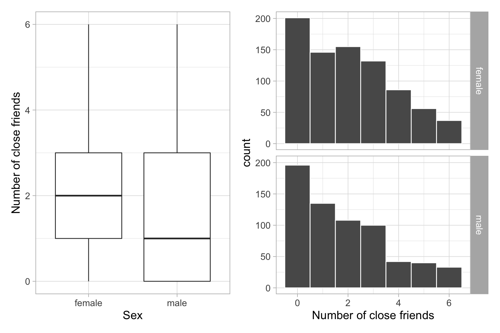

The distribution of number of close friends for both males and females appears to be skewed to the right. The variability in the number of close friends seems to be similar across males and females. The sample mean number of close friends seems to be slightly higher for females than males.

The sample mean number of close friends for females is \(\bar{x}_f\) = 2.09, with standard deviation \(s_f\) = 1.76 friends.

For males, the sample mean number of close friends is \(\bar{x}_m\) = 1.86, with standard deviation \(s_m\) = 1.78 friends.

The difference in sample means is \(\bar{x}_f - \bar{x}_m\) = 0.23.

Due to sampling variability, we can not conclude that, because the sample means differ, the means of the two populations must differ too.

We must resort to a principled framework to test this, and we have already learned to use statistical hypothesis testing in order to assess if sample results (in our case, the observed difference in sample mean number of close friends) are significant in the sense of being unlikely to have occurred by chance (from random sampling) alone.

Hypothesis test

We can perform a t-test either (a) by hand or (b) using built-in functions that automate all the computations. However, (a) is important to understand how the t-test works, so we will check (a) before showing the faster and completely equivalent way in (b).

(a) step-by-step calculations

We can use the table of summary statistics to calculate the value of the \(t\)-statistic.

Let’s extract the relevant statistics from the table of descriptive summaries:

n_f <- filter(descr_stats, sex == 'female') %>% pull(SampleSize)
n_m <- filter(descr_stats, sex == 'male') %>% pull(SampleSize)

xbar_f <- filter(descr_stats, sex == 'female') %>% pull(Mean)
xbar_m <- filter(descr_stats, sex == 'male') %>% pull(Mean)

s_f <- filter(descr_stats, sex == 'female') %>% pull(SD)
s_m <- filter(descr_stats, sex == 'male') %>% pull(SD)

Step 1. Can the population variances be assumed equal? Test the following hypotheses:

\[ H_0 : \sigma_f^2 = \sigma_m^2 \\ H_1 : \sigma_f^2 \neq \sigma_m^2 \]

or, equivalently: \[ H_0 : \frac{\sigma_f^2}{\sigma_m^2} = 1 \\ H_1 : \frac{\sigma_f^2}{\sigma_m^2} \neq 1 \]

Use the F-test to test for equality of the population variances:

var.test(num_close_friends ~ sex, data = gss)

## 
##  F test to compare two variances
## 
## data:  num_close_friends by sex
## F = 0.98094, num df = 812, denom df = 653, p-value = 0.7937
## alternative hypothesis: true ratio of variances is not equal to 1
## 95 percent confidence interval:
##  0.847352 1.134264
## sample estimates:
## ratio of variances 
##          0.9809412

At a significance level of 0.05, the \(p\)-value = 0.79 leads us to not reject the null hypothesis of equal variances across the two populations.

Step 2. We can now perform the \(t\)-test calculations using the appropriate formula for the standard error of the difference in means. As the population variances are assumed equal, we use the formula involving the pooled standard deviation:

# Pooled SD
s_p <- sqrt(
  ((n_f - 1) * s_f^2 + (n_m - 1) * s_m^2) / (n_f + n_m - 2)
)

SE <- s_p * sqrt(1/n_f + 1/n_m)

t_obs <- (xbar_f - xbar_m) / SE
t_obs

## [1] 2.4523

We reach to a conclusion about our hypothesis test either via the

• critical value approach: Compare the observed \(t\)-statistic with the appropriate 5% critical value(s) from a \(t\)-distribution.

• p-value approach: Compare the \(p\)-value with the significance level \(\alpha = 0.05\).

Critical value approach

tstar <- qt(c(0.025, 0.975), df = n_f + n_m - 2)
tstar

## [1] -1.961585  1.961585

Side note: As you can see, the t-distribution is symmetric. The value that cuts an area of 0.025 to its left, \(-t^* = -1.961585\) is equal to minus the value that cuts an area of 0.025 to its right, \(+t^* = 1.961585\) \[ -t^* = -( +t^* ) \]

Is the observed t-statistic more extreme than the critical values?

t_obs <= tstar[1]

## [1] FALSE

t_obs >= tstar[2]

## [1] TRUE

The observed t-statistic 2.45 is larger than the upper critical value 1.96. Hence, at the 5% significance level we have sufficient evidence against the null hypothesis that males and females have the same number of close friends.

\(p\)-value approach

p_value <- 2 * (1 - pt(t_obs, df = n_f + n_m - 2))
p_value

## [1] 0.01431058

At a 5% significance level, the observed difference in mean number of close friends between adult American females and males is significantly different from 0 (\(t(1465) = 2.45\), \(p = 0.01\), two-tailed).

In other words, an observed difference in sample mean number of close friends of 0.23 is highly unlikely to occur by chance alone.

The sample data provide very strong evidence that, on average, adult American females and males tend to not have the same number of close friends.

If you want to visualise where the observed t-statistic lies on the t-distribution, as well as the critical values (in red), you can use the following code:

plot_x <- seq(-3, 3, by = 0.01)
plot_y <- dt(plot_x, df = n_f + n_m - 2)
plot_df <- tibble(plot_x, plot_y)
plot_df

## # A tibble: 601 × 2
##    plot_x  plot_y
##     <dbl>   <dbl>
##  1  -3    0.00448
##  2  -2.99 0.00461
##  3  -2.98 0.00475
##  4  -2.97 0.00490
##  5  -2.96 0.00504
##  6  -2.95 0.00519
##  7  -2.94 0.00535
##  8  -2.93 0.00551
##  9  -2.92 0.00567
## 10  -2.91 0.00584
## # … with 591 more rows

ggplot(plot_df, aes(x = plot_x, y = plot_y))+
    geom_line() +
    geom_vline(xintercept = t_obs, color = 'darkolivegreen4') +
    geom_vline(xintercept = tstar, color = 'red') +
    labs(x = 'Difference in means', y = 't density')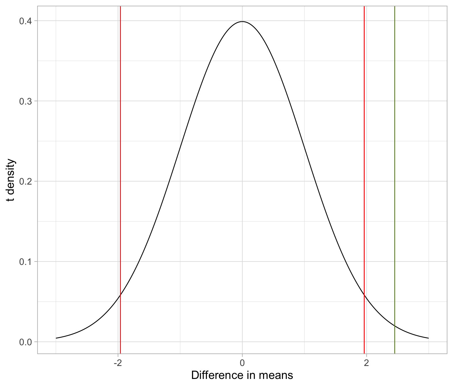

(b) built-in R function

In R, we can also perform a two-sample \(t\)-test very quickly using the function t.test. This is the same function you saw to perform a one-sample mean test.

Before applying it though, we need to check with var.test whether to assume the population variances to be different or equal.

Both R functions require a formula as first argument: goal( y ~ x )

where

• y is the response variable
• x is the explanatory variable
  
  

Step 1. Test for equality of the population variances. This is important so that later we know whether to set var = TRUE or var = FALSE in the function t.test():

var.test(num_close_friends ~ sex, data = gss)

Step 2. According to the previous test, use the appropriate \(t\)-test using either one of the following code chunks.

1. If you can not reject the null hypothesis of equal population variances, use a \(t\)-distribution with \(n_1 + n_2 - 2\) degrees of freedom:

t.test(num_close_friends ~ sex, data = gss, var.equal = TRUE)

2. If the population variances were not equal, we would have used the Welch-Satterthwaite approximation to the degrees of freedom:

# Welch-Satterthwaite approximation
t.test(num_close_friends ~ sex, data = gss, var.equal = FALSE)

# If not provided, var.equal = FALSE by default
t.test(num_close_friends ~ sex, data = gss)

We have already tested before for equality of the population variances:

var.test(num_close_friends ~ sex, data = gss)

## 
##  F test to compare two variances
## 
## data:  num_close_friends by sex
## F = 0.98094, num df = 812, denom df = 653, p-value = 0.7937
## alternative hypothesis: true ratio of variances is not equal to 1
## 95 percent confidence interval:
##  0.847352 1.134264
## sample estimates:
## ratio of variances 
##          0.9809412

As we cannot reject the null hypothesis of equal variances across the two populations, we use a \(t\)-test with \(\textrm{df} = n_1 + n_2 - 2\), i.e. we set var.equal = TRUE:

t.test(num_close_friends ~ sex, data = gss, var.equal = TRUE)

## 
##  Two Sample t-test
## 
## data:  num_close_friends by sex
## t = 2.4523, df = 1465, p-value = 0.01431
## alternative hypothesis: true difference in means between group female and group male is not equal to 0
## 95 percent confidence interval:
##  0.04556467 0.40984457
## sample estimates:
## mean in group female   mean in group male 
##             2.088561             1.860856

The independent sample t-test has the following assumptions:

• Independence of observations within and across groups.
• Continuous variable is approximately normally distribution within both groups.
  • Equivalently, that the difference in means is normally distributed.
• Homogeneity of variance across groups.

Let’s check them:

• The data were collected from a random sample of adult Americans.
• Even though the distribution of the number of close friends is clearly skewed, the sample sizes (813 and 654) are quite large. For large sample sizes, we know that the distribution of the difference in means will be normal.
• The result of the F-test for equality of the two variances indicates that fail to reject the null hypothesis of equal variances.

Hence, the conditions required for the two-sample \(t\)-test results to be valid are satisfied.

Now that we have established that there is significant evidence of a difference in the population mean number of close friends between females and males, how much do they actually differ??? In other words, what is the magnitude of this difference in the population means?

We can construct and interpret a 95% confidence interval for the difference in population mean number of close friends between females and males. We also need to pay particular attention on whether the interval is negative, positive, or contains zero.

In order to estimate the magnitude of the difference in the population means we can use a confidence interval for the difference in means:

ci <- (xbar_f - xbar_m) + tstar * SE
ci

## [1] 0.04556467 0.40984457

Note that the same result is given by the t.test() function in these lines of the output

## 95 percent confidence interval:
##  0.04556467 0.40984457

A 95% confidence interval for the difference in the mean number of close friends between females and males is [0.046, 0.41].

The confidence interval is entirely positive, supporting our conclusion that females and males tend to differ with regard to the average number of close friends.

We are 95% confident that American females have between 0.046 and 0.41 more close friends, on average, than American males do.

The sample results are significant, and we can also compute the effect size to check whether or not they are important.

library(effsize)
cohen.d(num_close_friends ~ sex, data = gss, mu = 0, pooled = TRUE)

## 
## Cohen's d
## 
## d estimate: 0.1288115 (negligible)
## 95 percent confidence interval:
##      lower      upper 
## 0.02567019 0.23195278

or

cohen.d(gss$num_close_friends, gss$sex, mu = 0, pooled = TRUE)

## 
## Cohen's d
## 
## d estimate: 0.1288115 (negligible)
## 95 percent confidence interval:
##      lower      upper 
## 0.02567019 0.23195278

As you can see above, the effect size, while being significant, is deemed to be of negligible importance.

Causation: Do the data provide evidence that how many close friends one has is caused by ones’ sex?

No, we can not conclude that the person’s sex was responsible for the number of close friends. This data was collected as part of an observational study, hence the explanatory variable sex was simply observed in the observational units.

Generalisation: To which population can the results of this study be applied to?

Because the observational units are a random sample from the population of adult Americans in year 2004, we might apply our results to adult American men and women in that year.

We might hesitate in generalising the results to all Americans and to a different year, as younger people were not included in the survey, and because the trend could have changed over time.

Exercises: Does name increase tips?

Think about it

• Can a server earn higher tips simply by introducing themselves by name when greeting customers?
• How can they investigate this?
• After data are collected, how can they decide if the results provide convincing evidence that giving their name does really lead to higher tips?
• And if they decided that introducing themself by name really helps, how can they estimate how much higher will the tips be, on average, when introducing themself by name?

The published experiment

Researchers Garrity and Degelman (1990) investigated the effect of a server introducing themself by name on restaurant tipping. The study involved forty, 2-person parties eating a $23.21 fixed-price buffet Sunday brunch at Charley Brown’s Restaurant in Huntington Beach, California, on April 10 and 17, 1988. Each two-person party was randomly assigned by the server to either a name or a no name introduction condition using a random mechanism. The server kept track of the two-person party condition and how much the party tipped at the end of the meal.

The published data

The paper provides very limited information about the data, i.e. only summary statistics and not the individual measurements. For this reason, you won’t be able to use the t.test() function, which requires the actual data. You will have to compute the t-statistic using the formulas.

• The sample mean tip for the 20 parties in the name condition was \(\bar x_{name}= \$5.44\), with a standard deviation \(s_{name} = \$1.75\).

• For the 20 parties in the no name condition, the sample mean tip was \(\bar x_{no\ name}= \$3.49\), with a standard deviation \(s_{no\ name} = \$1.13\).

Question 1

Identify the observational units in this study.

Solution

The observational units are the forty 2-person parties eating Sunday brunch in that restaurant on April 10 and 17, 1988.

We can also refer to the observational units as experimental units because, as we will see later, they are part of an experiment.

Question 2

Is this an observational study or a randomized experiment? Explain why.

Solution

This study is a randomized experiment. The server used a random mechanism to assign the experimental units (the two-person parties) either to a name or no name condition.

We also need to keep in mind that the server was not blind to which condition each party was assigned to and might have inadvertently provided better service to the parties they expected to give them a larger tip.

Question 3

What are the explanatory and response variables in this study?

Classify them as either categorical (also binary) or quantitative.

Solution

• Explanatory variable: condition (name or no name).

  Type: categorical and binary.

• Response variable: tipping amount.

  Type: quantitative.

Question 4

State, in words and in symbols, the server’s null and alternative hypotheses.

Solution

The null hypothesis is that there is no effect on the tipping amount from the server giving their name as part of their greeting to the customers.

Equivalently, the null hypothesis states that the population mean tip amount is the same whether the server introduces themself by name or not.

The alternative hypothesis is that there is a positive effect on the tipping amount from the server giving their name as part of their greeting to the customers.

Equivalently, the alternative hypothesis states that the population mean tip amount is greater when the server introduces themself by name than when they does not.

In symbols, \[ H_0 : \mu_{name} = \mu_{no\ name} \\ H_1 : \mu_{name} > \mu_{no\ name} \]

Question 5

Comment on what a Type I error and a Type II error would mean in this particular study.

Would you consider one of these two errors to be more worrying than the other? Explain why.

Solution

A Type I error is committed when the server decides that introducing themself by name helps when, in reality, it does not.

A Type II error is committed when the server decides that introducing themself by name is not helpful when, in reality, it actually is.

A Type I error means that the server will spend just a tiny amount of time longer as part of their greeting without getting any extra benefit from it.

A Type II error means that the server will not bother giving customers their name and thus would lose out on a higher tip.

Clearly, as the burden of adding the name to the introduction is minimal, we consider as more worrying (or worst error) losing out on potential tips. So, in this specific study, a Type II error is of higher concern.

Question 6

Assuming that the population variances are not equal, calculate the test statistic and the \(p\)-value. Note that this requires using the Welch t-test.

For your convenience, we have already calculated the degrees of freedom, which are \(\textrm{df} =\) 32.5.

Hint: As you do not have the party-by-party tipping amounts, but only summary statistics, you can not use the t.test() function, which requires the data at the finest level (the observational units).

Solution

The two-sample \(t\)-test in the case of unequal population variances involves the Welch-Satterthwaite approximation to the degrees of freedom.

The \(t\)-statistic is:

n_name <- 20
xbar_name <- 5.44
s_name <- 1.75

n_no <- 20
xbar_no <- 3.49
s_no <- 1.13

SE <- sqrt(s_name^2 / n_name + s_no^2 / n_no)
t_obs <- (xbar_name - xbar_no) / SE
t_obs

## [1] 4.186343

The question provides us the degrees of freedom calculated using Welch’s formula: \(\textrm{df} = 32.5\).

df <- 32.5

Critical value:

qt(0.95, df = df)

## [1] 1.693112

\(p\)-value:

pvalue <- 1 - pt(t_obs, df = df)
pvalue

## [1] 0.0001010876

The p-value is \(< .001\).

Question 7

At the significance level \(\alpha = 0.05\), what would you conclude?

Solution

As \(p < .001\), we reject the null hypothesis that there is no effect of introducing yourself by name on customers’ tipping amount.

The sample results provide strong evidence that including your name as part of the customer’s greeting tends to lead to higher tips on average.

Question 8

The paper only reports the sample mean tips and standard deviations for the name and no name conditions.

Does the paper provide enough information to check whether the validity conditions of the two-sample t-test are satisfied?

If yes, check that the conditions are met. If not, explain which additional information you would need.

Solution

We do not have enough information to check whether the validity conditions are met.

We are told that the two-person parties were randomly assigned either to the name or no name condition, but the two sample sizes (20 and 20) are not very large, so we should check whether the data came from normal distributions.

However, we only have summary statistics and not the actual tip amounts for each party (experimental unit). We would ask the server to provide us the party-by-party tipping amounts in order to check if the populations the samples came from can be assumed to be normal.

Question 9

Calculate a 95% confidence interval for the difference in population mean tipping amount between the name and no name conditions.

Write a sentence or two interpreting what the interval reveals.

Hint: The degrees of freedom were given in Question 6.

Solution

First, we must find the appropriate critical values \(\pm t^*\) (for the desired confidence level) from a t-distribution with degrees of freedom given by Welch’s method (see Question 6 for the value).

The upper critical value for a 95% confidence level is:

tstar <- qt(c(0.025, 0.975), df)
tstar

## [1] -2.035705  2.035705

We compute a 95% confidence interval for the difference in population means, \(\mu_{name} - \mu_{no\ name}\), as follows: \[ (\bar x_{name} - \bar x_{no\ name}) \pm t^* \ \sqrt{\frac{s_{name}^2}{n_{name}} + \frac{s_{no\ name}^2}{n_{no\ name}}} \\ (5.44 - 3.49) \pm 2.036 \ \sqrt{\frac{1.75^2}{20} + \frac{1.13^2}{20}} \]

SE <- sqrt(s_name^2 / 20 + s_no^2 / 20)

ci <- (xbar_name - xbar_no) + tstar * SE
ci

## [1] 1.001768 2.898232

The 95% confidence interval is [1, 2.9].

We are 95% confident that the server would earn, on average, between $1 and $2.9 more per party with a $23.21 bill, by including their name as part of the greeting.

Question 10

Regardless of whether the validity conditions of the t-test are met, summarise your conclusions from this test.

Make sure to also comment on causation and generalisability of your results.

Solution

The study involved random assignment of the experimental units to the groups, so the only difference between the groups was whether the party was given the server’s name or not. As the parties in the name condition tend to give significantly higher tips on average than those in the no name condition (\(t(32.5)\) = 4.19, \(p < .001\), one-sided), we can attribute this difference in means to being told the server’s name as part of the greeting. In other words, we can conclude a causal link between being given the name as part of the greeting and receiving higher tips on average.

However, as the server was not blind to the treatment condition, we must be wary to the fact that the server could have given better service to the parties who they gave their name to. So, the results hold unless the server gave better service to the name condition.

Having established that there is a significant difference in means between the two groups, a confidence intervals lets us now to estimate, on average, how much higher the tips will be when giving their name. Including their name as part of the greeting to customers increases the server’s tips, on average, by $1 to $2.9 per party.

We must be careful when generalising these results to the population. As only one particular server participated in the study, we don’t want to generalise these results to other servers. Furthermore, we might also avoid generalising these results to customers different from those who eat Sunday brunch at Charley Brown’s Restaurant in Huntington Beach, California.

Finally, the p-values and confidence interval are valid only if the response variable “tipping amount” is normally distributed in the two populations.

References

• Garrity, K., & Degelman, D. (1990). Effect of server introduction on restaurant tipping. Journal of Applied Social Psychology, 20(2), 168-172.
• Rossman, A. J., & Chance, B. L. (2011). Workshop statistics: discovery with data. John Wiley & Sons.