Paired sample t-test

1. To understand the t-test for paired samples
2. Learn how to compute Cohen’s \(D\) for different types of t-test.
3. Be able to report the results of paired-sample t-test

One of the assumptions of the t-test is that the data are independently sampled. Sometimes this assumptions does not hold. A clear example is the case of paired data. These may consist of two measurements on each unit, such as the same unit being measured under two different conditions, or measurements on a pair of units that go together, such as twin studies.

The paired sample t-test (also known as the “dependent samples t-test”) is used in scenarios such as:

• Same units observed on two occasions: A measurement is taken on the same subject before and after some treatment, or at two different timepoints - e.g. response times to a task before and after ingesting a caffeine drink.

• Same units observed on a pair of variables: A measurement is taken under two different conditions - e.g. response time of the same subject is measured on two different drugs.

• Pairs of people: A measurement is taken of the same variable but from different people from a dyad (pair of people) - e.g. do store employees work different amount of hours to their bosses?

In all these scenarios, we are interested in comparing the measurements between two groups in which each observation in one group can be paired with an observation in the other group.

The following table gives an example where 10 subjects have their heartbeats per minute measured in two occasions, in the morning (\(HB_M\)) and in the afternoon (\(HB_A\)) . \[ \begin{matrix} \text{Subject} & HB_M & HB_A \\ 1 & 71 & 83 \\ 2 & 64 & 78 \\ \vdots & \vdots & \vdots \\ 10 & 85 & 97 \end{matrix} \]

Clearly the data aren’t independent. Some people might typically have higher heartbeats than others, and for this reason the data corresponding to the same subject are dependent. However, the data between different people should be independent.

We can get rid of the by-subject dependence by computing, for each subject, the difference!

\[ \begin{matrix} \text{Subject} & HB_M & HB_A & d = HB_A - HB_M \\ 1 & 71 & 83 & 12 \\ 2 & 64 & 78 & 14 \\ \vdots & \vdots & \vdots & \vdots \\ 10 & 85 & 97 & 12 \end{matrix} \]

and we are interested in whether the difference is, on average, equal to some hypothesised value, such as 0 for example. If this were the case, on average the heartbeats in the morning would be the same as the heartbeats in the afternoon.

The paired t-test

Null hypothesis

A paired sample t-test has a familiar null hypothesis:

\[H_0: \mu_d = 0\]

i.e. the population mean difference is 0.

Alternative hypotheses

The alternative hypotheses can be two-sided, or one-sided (left-tailed or right-tailed).

• (two-sided) \(H_1 : \mu_d \neq 0\) (the population mean difference is 0)
• (left-tailed) \(H_1 : \mu_d < 0\) (the population mean difference is smaller than 0)
• (right-sided) \(H_1 : \mu_d > 0\) (the population mean difference is greater than 0)

But what does that mean that the population mean difference is smaller (larger) than 0? It means that the measurements in group 1 are, on average, smaller (larger) than group 2.

Test statistic

\[ t_{obs} = \frac{\bar{d}}{SE}, \qquad \text{where } SE = \frac{s_d}{\sqrt{n}} \]

in the formula above:

• \(\bar{d}\) = sample mean of the differences
• \(s_d\) = sample standard deviation of the differences
• \(n\) = sample size (number of unique pairs)

Confidence interval

A 95% confidence interval for the population mean difference \(\mu_d\) is:

\[ \bar{d} \pm t^* \cdot SE \] where

• \(\bar{d}\) is the mean of the differences in the sample
• \(\pm t^*\) are the appropriate quantiles of a t-distribution with \(n - 1\) degrees of freedom
• \(SE = \frac{s_d}{\sqrt{n}}\) is the standard error of the mean (of the differences)

Note: For a 99% confidence interval, remember to change the quantile to \(t_{0.995}\)!

Assumptions

For the results of a paired t-test to be valid, the following assumptions should be met:

1. Your dependent variable (DV) is measured on a numeric scale (discrete/continuous level)
2. Your independent variable (IV) should consist of two categorical, ‘matched pairs’ (see example above)
3. The differences between the pairs should be approximately normally distributed (i.e. the distribution of the differences in the DV between the two groups)
4. There should be no extreme outliers in the differences

Checking assumptions

1. This is a design issue - which level of data should be confirmed before data collection/during study design period.
2. This is a design issue.
3. This can be tested using the Shapiro-Wilk test of normality and/or also assessed visually with plots (such as histograms and density plots). A QQplot can also be used.
4. Outliers can be identified using boxplots. The indentify_outliers() function in the rstatix package can extract rows suspected as outliers.

One sample t-test in disguise

The paired-sample t-test is very similar to the one sample t-test covered in Week 7.

The steps for the one sample t-test are:

1. calculate the sample mean (\(\bar{x}\))

2. calculate the sample standard deviation \(s\) of the data \(x_i\)

3. calculate the standard error \(SE = \frac{s}{\sqrt{n}}\)

4. calculate \(t_{obs} = \frac{\text{estimate} - \text{null}}{SE} = \frac{\bar{x} - \mu_0}{SE}\)

5. calculate the probability of observing a \(t\)-statistic at least as extreme, assuming the null hypothesis (\(H_0: \mu = \mu_0\)) is true.

The steps for the paired t-test are:

1. calculate the difference score for each pair: \(d_i = x_{i1} - x_{i2}\)

2. calculate the sample mean of the differences: \(\bar{d} = \sum d_i / n\)

3. calculate the sample standard deviation of the differences, and denoted it \(s_d\)

4. calculate the standard error \(SE = \frac{s_d}{\sqrt{n}}\)

5. calculate \(t_{obs} = \frac{\text{estimate} - \text{null}}{SE} = \frac{\bar{d} - \mu_0}{SE}\)

6. calculate the probability of observing a \(t\)-statistic at least as extreme, assuming the null hypothesis (\(H_0: \mu_d = \mu_0\)) is true.

Typically, the hypothesised value \(\mu_0\) is equal to 0. The formula for the t-statistic, assessing statistical significance, and constructing confidence intervals is identical to the one-sample t-test.

We have just changed the notation - instead of talking about a population mean \(\mu\) of a variable \(x\), which is estimated by a sample mean (\(\bar{x}\)), we are talking about a population mean of differences (\(\mu_d\)) which is estimated by the sample mean of the differences (\(\bar{d}\)). We are testing whether the population mean difference (\(\mu_d\)) is different from 0.

Questions

Change in score on the ACE-III

Addenbrooke’s Cognitive Examination-III (ACE-III) is a brief cognitive test that assesses five cognitive domains: attention, memory, verbal fluency, language and visuospatial abilities. The total score is 100 with higher scores indicating better cognitive functioning. A research project is examining changes in cognitive functioning with age, and administers the ACE-III to a set of participants at age 60, then again at age 70.

How is the data from this study paired?

The same people have the same variable (ACE-III score) measured at different time points (age 60 then age 70).

Hypotheses

Now, we write the null and alternative hypothesis:

As the research project is examining ‘changes’ without specifying which direction, we can write a null hypothesis and a two-sided alternative hypothesis.

Our null hypothesis is that the population means in scores on the ACE-III between ages 60 and 70 are the same (i.e. no change/the difference in means is = 0).

Our alternative hypothesis is that the population means in scores on the ACE-III between ages 60 and 70 is not equal (i.e. scores at age 70 are different from scores at age 60).

By taking the difference in the cognitive scores at age 70 and 60, we can assess this by testing whether

\[ H_0: \mu_d = 0 \\ H_1: \mu_d \neq 0 \]

Read in the data

Next, we read in the data and make a new column of the difference in scores for each pair.

acedata <- read_csv("https://uoepsy.github.io/data/acedata.csv")

acedata <- acedata %>%
  mutate(diff_score = ace_70 - ace_60)

head(acedata) # look at the "head" of the data frame 

## # A tibble: 6 × 4
##   participant ace_60 ace_70 diff_score
##   <chr>        <dbl>  <dbl>      <dbl>
## 1 sub1            93     85         -8
## 2 sub2            95     92         -3
## 3 sub3            93     90         -3
## 4 sub4            93     95          2
## 5 sub5            96     88         -8
## 6 sub6            91     85         -6

Performing a one-sample t-test

To assess if there is a significant difference in ACE-III scores for particpants at ages 60 and 70, we must calculate the mean difference (\(\bar{d}\)), our sample standard deviation (\(s_d\)) and our sample size (\(n\)).

aceterms <- acedata %>% 
  summarise(
    dbar = mean(diff_score),
    s_d = sd(diff_score),
    n = n()
  )

aceterms

## # A tibble: 1 × 3
##    dbar   s_d     n
##   <dbl> <dbl> <int>
## 1 -2.48  5.50    25

Calculate the t-statistic

Let’s recall the formula for the observed t-statistic: \[ t_{obs} = \frac{\bar d - 0}{SE}, \qquad \text{where} \qquad SE = \frac{s_d}{\sqrt n} \]

In R:

SE <- aceterms$s_d / sqrt(aceterms$n)
t_stat <- (aceterms$dbar - 0) / SE
t_stat

## [1] -2.254173

Calculate the p-value

The t-statistic is negative, so we can make it positive via abs(t_stat) and then compute it as twice the proportion as larger as, or larger than, abs(t_stat):

2 * (1 - pt(abs(t_stat), df = 24))

## [1] 0.03358854

Equivalently, you could have computed it as:

2 * pt(abs(t_stat), df = 24, lower.tail = FALSE)

## [1] 0.03358854

Calculate the 95% confidence interval

# mean difference between measurements
aceterms$dbar

## [1] -2.48

# standard error
SE <- aceterms$s_d / sqrt(aceterms$n)
SE

## [1] 1.100182

# tstar
tstar <- qt(c(.025, .975), df = 24) 
tstar

## [1] -2.063899  2.063899

ci <- aceterms$dbar + tstar * SE
ci

## [1] -4.7506636 -0.2093364

What does all this mean?

At the 5% significance level, we performed a paired sample t-test to determine whether cognitive functioning ¹ differs, on average, between the ages of 60 and 70 (\(t(24) = -2.25, p = .034\), two-tailed).

The mean difference in ACE-III scores for ages 70 and 60 is -2.48 (95% CI [-4.75, -0.21]). The small p-value (0.034) indicates that if the difference in cognitive scores was, on average, truly equal zero, we would expect to observe a sample difference as large as -2.48 only in 3 samples out of 100. Hence, the sample data provide strong evidence against the null hypothesis and in favour of the alternative that the difference is cognitive scores is on average different from zero.

However, the result of the t-test doesn’t help us interpret whether cognitive scores are higher at 60 or 70 years. To understand that, we interpret the confidence interval paying particular attention to whether it is entirely positive or negative.

A 95% confidence interval for the difference in cognitive scores at 70 and 60 years is [ -4.75 -0.21]. We are 95% confidence that at 70 years the cognitive score is, on average, between 0.21 and 4.75 less than at 60 years.

In one function

t.test(acedata$ace_70, acedata$ace_60, paired = TRUE) # remember the default setting is two-sided

## 
##  Paired t-test
## 
## data:  acedata$ace_70 and acedata$ace_60
## t = -2.2542, df = 24, p-value = 0.03359
## alternative hypothesis: true difference in means is not equal to 0
## 95 percent confidence interval:
##  -4.7506636 -0.2093364
## sample estimates:
## mean of the differences 
##                   -2.48

Looks like all the values match up!

Reshaping data frames

Your data frames can be reshaped from ‘wide’ to ‘long’ formats, and vice versa. What’s the difference?

Wide data is where you have repeated measurements in separate columns of the same record i.e. what the acedata currently is.

head(acedata)

## # A tibble: 6 × 4
##   participant ace_60 ace_70 diff_score
##   <chr>        <dbl>  <dbl>      <dbl>
## 1 sub1            93     85         -8
## 2 sub2            95     92         -3
## 3 sub3            93     90         -3
## 4 sub4            93     95          2
## 5 sub5            96     88         -8
## 6 sub6            91     85         -6

As we can see, there are separate columns for age_60 and age_70 and each participant has one row.

In comparison, the long format has repeated measurements gathers columns into rows.

acedata_long <- acedata %>%
    pivot_longer(ace_60:ace_70, names_to = "age", values_to = "ace_score")

head(acedata_long)

## # A tibble: 6 × 4
##   participant diff_score age    ace_score
##   <chr>            <dbl> <chr>      <dbl>
## 1 sub1                -8 ace_60        93
## 2 sub1                -8 ace_70        85
## 3 sub2                -3 ace_60        95
## 4 sub2                -3 ace_70        92
## 5 sub3                -3 ace_60        93
## 6 sub3                -3 ace_70        90

Now we can see that in the ‘participant’ column, each subject now has 2 rows - as the new column age has collapsed the age_60 and age_70 columns into a singular column.

The pivot_longer function used above too columns ace_60 to ace_70 (and anything in between), puts the names (variable names) into a new column called age, and puts the values into a column called ace_score.

t-test using long data

Now, we can run the same paired t-test using:

t.test(y ~ group, paired = TRUE, data = data)
t.test(data$y ~ data$group, paired = TRUE)

That is,

t.test(acedata_long$ace_score ~ acedata_long$age, paired = TRUE)

## 
##  Paired t-test
## 
## data:  acedata_long$ace_score by acedata_long$age
## t = 2.2542, df = 24, p-value = 0.03359
## alternative hypothesis: true difference in means is not equal to 0
## 95 percent confidence interval:
##  0.2093364 4.7506636
## sample estimates:
## mean of the differences 
##                    2.48

But wait… Why are the numbers different from what we had before???

Remember we computed the difference as ace_70 - ace_60. However, R doesn’t know if we want ace_70 - ace_60 or ace_60 - ace_70! R will always do the first level in alphabetical (ace_60 in this case) order - the second level in alphabetical order (ace_70 in this case).

If you want to do the other way around you need to swap the levels of the factor.

acedata_long$age <- as.factor(acedata_long$age)
levels(acedata_long$age)

## [1] "ace_60" "ace_70"

acedata_long$age <- fct_relevel(acedata_long$age, 'ace_70')
levels(acedata_long$age)

## [1] "ace_70" "ace_60"

t.test(acedata_long$ace_score ~ acedata_long$age, paired = TRUE)

## 
##  Paired t-test
## 
## data:  acedata_long$ace_score by acedata_long$age
## t = -2.2542, df = 24, p-value = 0.03359
## alternative hypothesis: true difference in means is not equal to 0
## 95 percent confidence interval:
##  -4.7506636 -0.2093364
## sample estimates:
## mean of the differences 
##                   -2.48

# equivalent
# t.test(ace_score ~ age, paired = TRUE, data = acedata_long)

There you go!!! Now R did ace_70 - ace_60.

Converting back to wide format

acedata_long %>%
    pivot_wider(names_from = age, values_from = ace_score)

## # A tibble: 25 × 4
##    participant diff_score ace_60 ace_70
##    <chr>            <dbl>  <dbl>  <dbl>
##  1 sub1                -8     93     85
##  2 sub2                -3     95     92
##  3 sub3                -3     93     90
##  4 sub4                 2     93     95
##  5 sub5                -8     96     88
##  6 sub6                -6     91     85
##  7 sub7                -2     94     92
##  8 sub8                 0     90     90
##  9 sub9                 2     90     92
## 10 sub10               -5     96     91
## # … with 15 more rows

Tah-dah! The age_60 and age_70 variables are back in their own columns :)

Plots

Visualising the data is always useful! Here, a boxplot is a good option as we can visualise the difference in means across the two time points.

ggplot(data = acedata_long, aes(x = age, y = ace_score)) +
    geom_boxplot()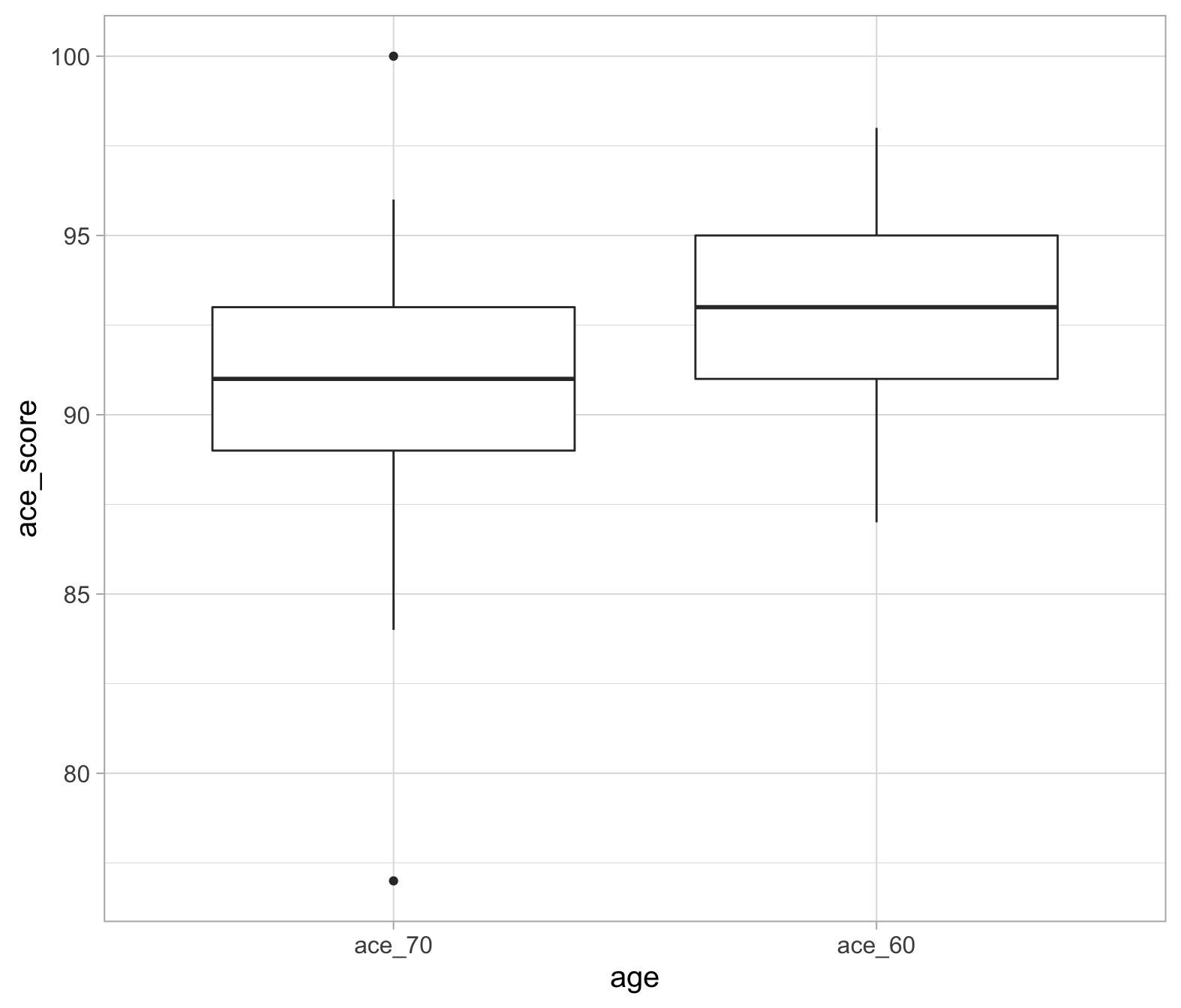

Note that we’re using the long data format here (see the optional box above if you skipped it!). We’re telling the ggplot function to put age on the x-axis and ace_score on the y axis. As age (x-axis) has two levels, it allows us to view the distributions of the ace_60 and ace_70 scores side-by-side.

Effect sizes

Cohen’s \(D\) is an effect size used to indicate the standardised difference between two means. For an interactive tool which allows you to change effect sizes, check out this link: https://rpsychologist.com/cohend/.

The formula for Cohen’s \(D\) are as follow for the different types of t-tests we’ve looked at:

Test	Cohen’s \(D\)
One-sample t-test	\(D = \frac{\bar{x} - 0}{s_x}\)
Independent samples t-test	\(D = \frac{(\bar{x}_1-\bar{x}_2) - 0}{s_p}\)
Paired t-test	\(D = \frac{\bar{d} - 0}{s_d}\)

Interpreting Cohen’s \(D\):

• approx. 0.2 = small effect
• approx. 0.5 = medium effect
• approx. 0.8 = large effect

Check out the link above with the interactive tool. Change the Cohen’s \(D\) to 0.2, 0.5 and 0.8 to compare the standardised differences between the two groups!

In practice, we already have the figures we need, stored in aceterms:

aceterms

## # A tibble: 1 × 3
##    dbar   s_d     n
##   <dbl> <dbl> <int>
## 1 -2.48  5.50    25

(aceterms$dbar - 0) / (aceterms$s_d)

## [1] -0.4508346

Look like we have a small-to-medium effect size.

Questions

Age differences in heterosexual marriages

Is there an age difference in heterosexual married couples (and in which direction)?

Data is available at: https://uoepsy.github.io/data/marriageages.csv

Question 1

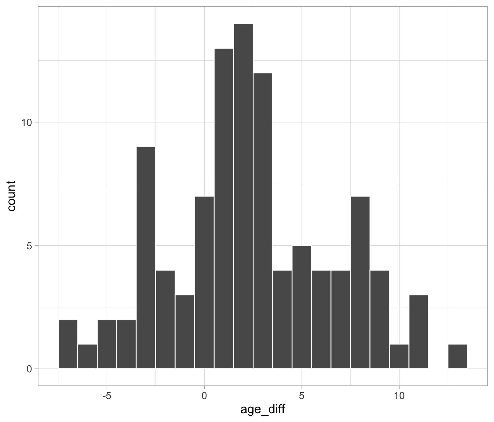
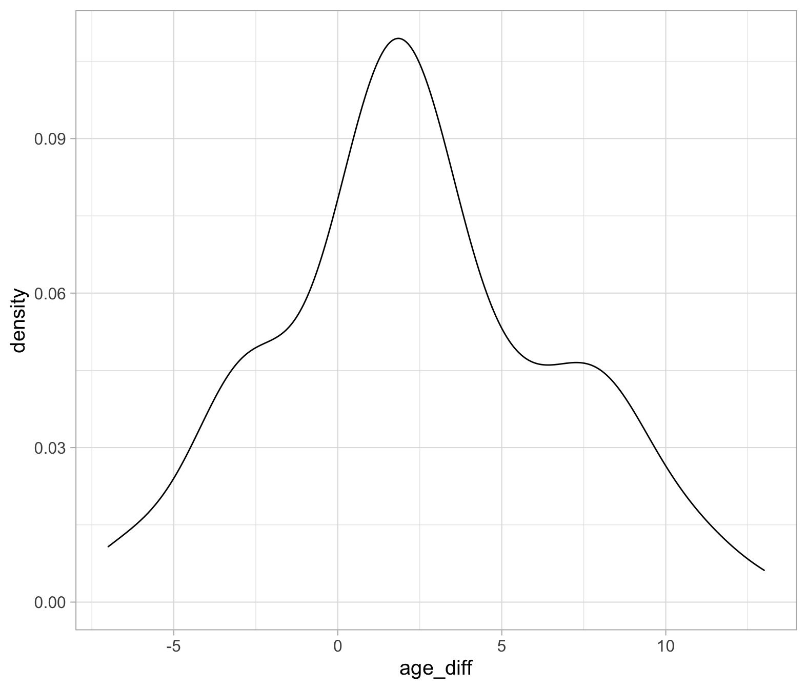
First, we must read in our data. Then, create a new column which is the husband’s age minus the wife’s age (i.e. the difference).

Solution

marriage_age <- read.csv("https://uoepsy.github.io/data/marriageages.csv")

marriage_age <- marriage_age %>%
    mutate(age_diff = Husband - Wife)
head(marriage_age)

##   Husband Wife age_diff
## 1      53   50        3
## 2      38   34        4
## 3      46   44        2
## 4      30   36       -6
## 5      31   23        8
## 6      26   31       -5

Question 2

As we are testing the differences, what assumptions are we making? And, what assumption checks can we do? (Remember, this is a one-sample t-test in disguise!)

Solution

As the repeated t-test is a one-sample t-test in disguise, we are assuming that the differences come from a normal distribution.

We can check this with visualisations, such as histograms and density plots:

ggplot(marriage_age, aes(x = age_diff)) +
    geom_histogram(binwidth = 1, color = 'white')

ggplot(marriage_age, aes(x = age_diff)) +
    geom_density()

We can also check using the shapiro.test() to test for normality:

shapiro.test(marriage_age$age_diff)

## 
##  Shapiro-Wilk normality test
## 
## data:  marriage_age$age_diff
## W = 0.98079, p-value = 0.1444

Remember, the Shapiro-Wilks test null hypothesis is that the distribution is normal (i.e. we want a non-significant p-value).

Looks like our data is consistent with the null hypothesis that the population is normally distributed!

Question 3

If we’re about to conduct a t-test on the difference scores, what will the results mean?

If we get a positive t-statistic \((t_{obs} > 0)\), what direction is the difference? I.e. who is older? The husbands or the wives?

Solution

As we calculated the Husband - Wife age, a positive t-statistic will indicate that this value is > 0. Therefore, our sample shows that the husbands tend to be older than the wives.

Question 4

Conduct a one-sample t-test, testing that the age differences are not equal to 0.

If you’re confused about one-sample t-tests, look back at Week 7’s lab!

Solution

t.test(marriage_age$age_diff, mu = 0)

## 
##  One Sample t-test
## 
## data:  marriage_age$age_diff
## t = 5.596, df = 101, p-value = 1.888e-07
## alternative hypothesis: true mean is not equal to 0
## 95 percent confidence interval:
##  1.531495 3.213603
## sample estimates:
## mean of x 
##  2.372549

Question 5

Now, run a t-test using the paired = TRUE argument of the t.test() function. Remember, as we have a column for husbands and a column for wives.

Compare the output with the output performed above - are they the same?

Solution

t.test(marriage_age$Husband, marriage_age$Wife, paired = TRUE)

## 
##  Paired t-test
## 
## data:  marriage_age$Husband and marriage_age$Wife
## t = 5.596, df = 101, p-value = 1.888e-07
## alternative hypothesis: true difference in means is not equal to 0
## 95 percent confidence interval:
##  1.531495 3.213603
## sample estimates:
## mean of the differences 
##                2.372549

Looks like they produce the same output! It really is a one-sample t-test in disguise.

Question 6

Calculate Cohen’s \(D\)

Solution

Recall the formula for Cohen’s \(D\) is: \[ D = \frac{\bar d - 0}{s_d} \]

Using R, you can compute it as:

mean(marriage_age$age_diff) / sd(marriage_age$age_diff)

## [1] 0.5540817

Or as a one-sample Cohen D but where the variable is the difference:

library(effsize)
cohen.d(marriage_age$age_diff, NA)

## 
## Cohen's d (single sample)
## 
## d estimate: 0.5540817 (medium)
## Reference mu: 0
## 95 percent confidence interval:
##     lower     upper 
## 0.1537776 0.9543857

cohen.d(marriage_age$Husband - marriage_age$Wife, NA)

## 
## Cohen's d (single sample)
## 
## d estimate: 0.5540817 (medium)
## Reference mu: 0
## 95 percent confidence interval:
##     lower     upper 
## 0.1537776 0.9543857

Question 7

Write a brief summary of the findings, using inline code (include mean ages, t-test output and Cohen’s \(D\)).

Solution

In our sample of married, heterosexual couples, the average age of the husbands is 33.92 (SD = 11.52), whilst the average age of the wives is 31.55 (SD = 10.41).

Based on our sample of heterosexual couples, the husband, on average, is 2.37 [95% CI 1.53, 3.21] years older than their wife and this difference is signficant \(t\)(101) = 5.6, \(p\) < .001. Further, Cohen’s effect size (\(D\) = 0.55) suggests a moderate effect.

Smoking interventions

A researcher has developed a cognitive behavioural therapy (CBT) based on a smartphone app, and is testing how effective it is in helping people to stop smoking.

The researcher recruited 60 participants who were trying to stop smoking. Over the course of a week, the researcher recorded the average number of cigarettes smoked per day, per participant. Thirty participants were given the app, and were asked every time they felt like smoking to open the app on and complete a five-minute task. All 60 participants were followed up a month later. The average number of cigarettes smoked per day (over a week) was recorded.

The data is available at: https://uoepsy.github.io/data/cbtsmoke.csv

Question 8

Read the data into R.

What was the average number of cigarettes smoked per day at both time-points for each group?

Solution

smoking <- read_csv("https://uoepsy.github.io/data/cbtsmoke.csv")

smoking %>%
    group_by(app_group) %>%
    summarise(
        initial = mean(cigs_pday),
        follow_up = mean(cigs_pday_1month)
    )

## # A tibble: 2 × 3
##   app_group initial follow_up
##   <chr>       <dbl>     <dbl>
## 1 no           14.8      12.7
## 2 yes          14.8       9.7

From the sample data, the average number of cigarettes smoked by the group which did not receive the app appears to be similar in the initial and follow-up time points.

The group which did receive the app, appears to have reduced their average consumption of cigarettes.

Question 9

At the point of recruitment, did the 60 participants smoke more or less than 20 cigarettes per day?

This is asking whether the mean number of cigarettes per day is different to 20. Thus, we are asking whether a mean is different from a hypothesised number i.e. a one-sample t-test!

P.S. Don’t forget to check your assumptions!

Solution

shapiro.test(smoking$cigs_pday) # checking our normality assumption 

## 
##  Shapiro-Wilk normality test
## 
## data:  smoking$cigs_pday
## W = 0.97845, p-value = 0.3666

At the 5% significance level, we performed a Shapiro-Wilk test against the null that the data came from a normal distribution. The large p-value (\(p = .37\)) indicates that we do not have sufficient evidence to reject the null hypothesis. Thus, our data are consistent with a normal population and we can go ahead to perform the one-sample t-test.

t.test(smoking$cigs_pday, mu = 20) # default is a two-sided alternative 

## 
##  One Sample t-test
## 
## data:  smoking$cigs_pday
## t = -11.095, df = 59, p-value = 4.544e-16
## alternative hypothesis: true mean is not equal to 20
## 95 percent confidence interval:
##  13.86217 15.73783
## sample estimates:
## mean of x 
##      14.8

At the 5% significance level, we performed a two-sided, one-sample t-test against the null hypothesis that the mean number of cigarettes smoked per day at the time of recruitment was equal to 20. (\(t\)(59) = -11.1, \(p\) < .001, two-sided.) The large t-statistic (-11.1) leads to a small p-value, indicating that we have very strong evidence against the null and in favour of the alternative that at time of recruitment the individuals did not smoke 20 cigaretts per day, on average.

Question 10

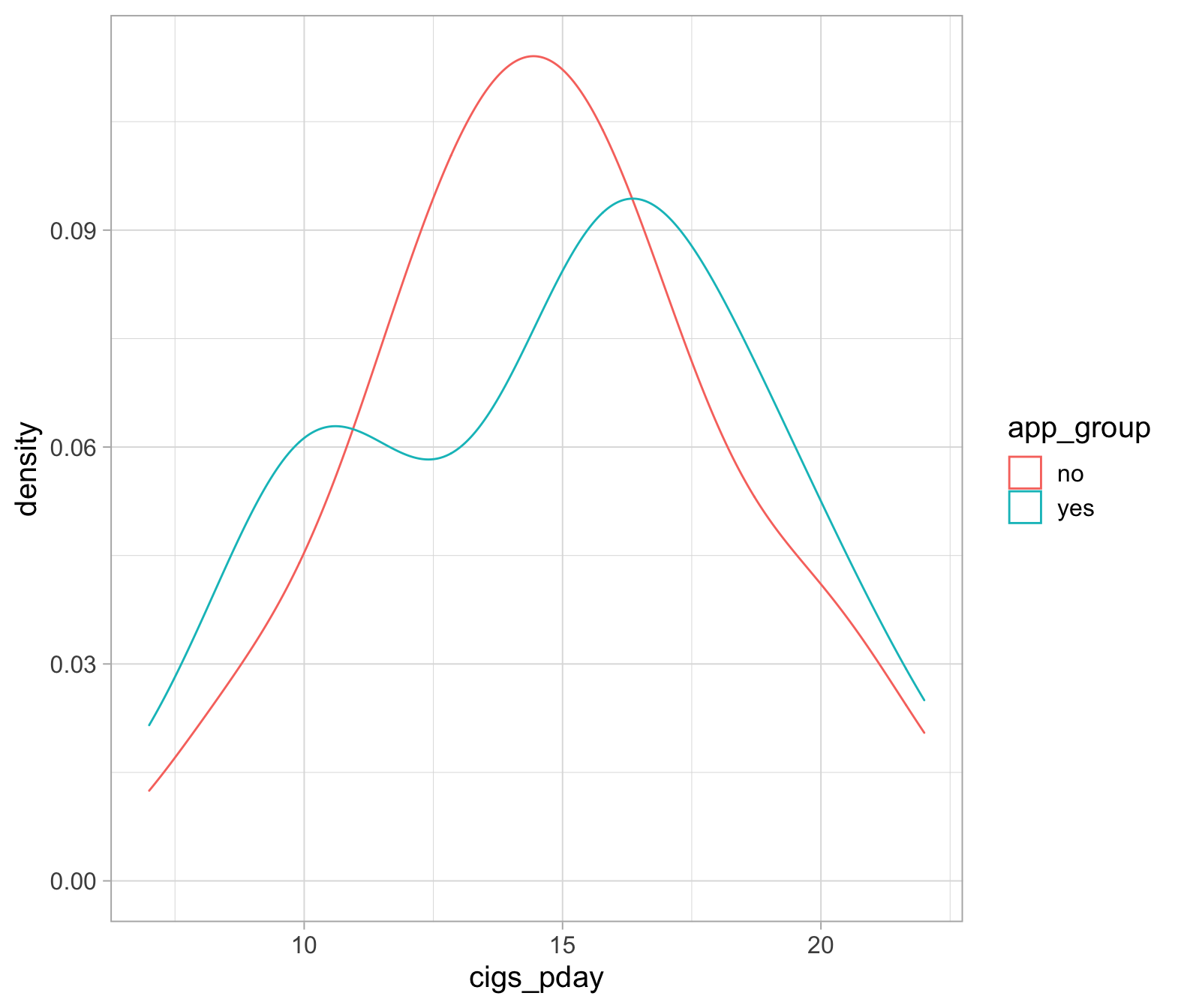
Did the average number of cigarettes smoked per day differ between the groups at the initial recruitment?

These observations (from the different groups) are independent, so we are going to perform an independent samples t-test.

And don’t forget, check your assumptions! (Look back to last weeks lab for independent sample t-tests if you’re stuck)

Solution

First, we need to check the assumption of equal variances between groups.

var.test(smoking$cigs_pday ~ smoking$app_group) # this function is looking at the variance of cigaretters smoked on average, predicted by the group

## 
##  F test to compare two variances
## 
## data:  smoking$cigs_pday by smoking$app_group
## F = 0.72721, num df = 29, denom df = 29, p-value = 0.3961
## alternative hypothesis: true ratio of variances is not equal to 1
## 95 percent confidence interval:
##  0.3461274 1.5278697
## sample estimates:
## ratio of variances 
##          0.7272121

Again, the null hypothesis for this test is that the variances are equal. As we have a p-value greater than our alpha level of 0.05, we fail to reject the null hypothesis and conclude the variances between groups are equal across the two populations.

It’s also worth checking our normality assumption. We can do this with visualisations such as histograms and density plots.

ggplot(smoking, aes(x = cigs_pday, col = app_group)) + # plotting average number of cigarettes smoked per day on the x-axis and giving different colours for each app group 
    geom_density() # telling R we want a density plot

All looks good (no skew and both look relatively normal), we can go ahead and perform the t-test.

t.test(smoking$cigs_pday ~ smoking$app_group, var.equal = TRUE)

## 
##  Two Sample t-test
## 
## data:  smoking$cigs_pday by smoking$app_group
## t = -0.070519, df = 58, p-value = 0.944
## alternative hypothesis: true difference in means between group no and group yes is not equal to 0
## 95 percent confidence interval:
##  -1.959022  1.825689
## sample estimates:
##  mean in group no mean in group yes 
##          14.76667          14.83333

We performed an independent samples-test to assess if there was a significant difference between the average number of cigarettes smoked per day between the groups at the initial time point. A two-sample t-test revealed there was no significant difference between the two groups \(t\)(58) = -0.07, \(p\) = 0.944, two-sided. Thus, the sample data do not provide enough evidence against the null hypothesis that the population mean difference is 0.

Question 11

Did the group given the app change their smoking habits from the intial time point to the one-month follow up? If so, was there a big change?

Here, we need to focus on the data from those who were given the app. The second question is asking about effect size.

Solution

As we’re only interested in the group given the app, we can create a new data set which only contains the participants assigned to the experimental condition.

smoking_app <- smoking %>%
    filter(app_group == "yes") # telling R we want to look inside the original data set 'smoking' and extract those with 'yes' in the app_group column 

Now, we can perform the paired-test.

Remember, the question is asking about the same participants: they provided data at two time points and we’re interested to see if there is a significant difference between these points.

t.test(smoking_app$cigs_pday, smoking_app$cigs_pday_1month, paired = TRUE)

## 
##  Paired t-test
## 
## data:  smoking_app$cigs_pday and smoking_app$cigs_pday_1month
## t = 5.0883, df = 29, p-value = 1.985e-05
## alternative hypothesis: true difference in means is not equal to 0
## 95 percent confidence interval:
##  3.070004 7.196663
## sample estimates:
## mean of the differences 
##                5.133333

Alternatively, you can address this question with a one-sample t-test, focusing on the difference scores.

smoking_app <- # overwriting the dataset which only contains participants assigned to the app condition and adding a new column which is the difference in cigarettes smoked at time point 1 and time point 2 
    smoking_app %>%
    mutate(difference = cigs_pday - cigs_pday_1month)

t.test(smoking_app$difference, mu = 0) # assessing if this difference is signficantly different from 0 

## 
##  One Sample t-test
## 
## data:  smoking_app$difference
## t = 5.0883, df = 29, p-value = 1.985e-05
## alternative hypothesis: true mean is not equal to 0
## 95 percent confidence interval:
##  3.070004 7.196663
## sample estimates:
## mean of x 
##  5.133333

Looks like the numbers from both variations of the t-test match up, wahoo!

The researchers were also interested in the effect size.

smoking_app %>%
    summarise(
        dbar = mean(difference),
        s = sd(difference)
    )

## # A tibble: 1 × 2
##    dbar     s
##   <dbl> <dbl>
## 1  5.13  5.53

5.133333/5.525698

## [1] 0.9289927

Writing-up

A paired-test was performed to assess if there was a significant difference in the average number of cigarettes smoked in participants who were in the experimental (app) condition. On average, compared to the initial timepoint (\(M\) = 14.83), participants smoked less cigarettes at the one-month follow-up (\(M\) = 9.70). This difference 5.13 [95% CI 3.01, 7.20], was statistically significant \(t\)(29) = 5.09, \(p\) < .001, two-sided. This difference between time points was large (\(d\) = 0.93).

---

1. as measured using the total scores on the ACE-III.↩︎