Chi-square tests

1. Understand when to use a chi-square goodness-of-fit test and chi-square test of independence
2. Check the assumptions for the tests
3. Report the test results

The past few weeks have focused on tests for numeric response variables, such as:

• a numeric response variable (one-sample t-test and paired t-test)
• a numeric response variable and binary categorical explanatory variable (paired t-test)

This week we will investigate tests for:

• a categorical response variable (\(\chi^2\) goodness-of-fit test);
• a categorical response variable and a categorical explanatory variable (\(\chi^2\) test of independence).

For the first time, you will be working with a statistical test that applies to categorical variables with more than two categories.

Note: the symbol \(\chi^2\) is also written as “chi-square” or “chi-squared,” and is pronounced “kai-square” or “kai-squared.”

The two tests of focus this week are the \(\chi^2\) goodness-of-fit test and the \(\chi^2\) test of independence. The first is used to assess whether sample results conform with an hypothesis about the proportional breakdown of the various categories in the population. The latter tests if two categorical variables are associated in the population or not.

Chi-square goodness-of-fit test

The \(\chi^2\) goodness-of-fit test applies to categorical variables. For ease of exposition, suppose the categorical variable of interest has \(C\) possible unique categories. For example, the variable “Days of the week” has \(C = 7\) possible categories: Monday, Tuesday, Wednesday, Thursday, Friday, Saturday, and Sunday.

We have collected sample data for a variable of interest, and we can compute the proportion of individuals in the sample falling into each of the \(C\) distinct categories, \(p_1, p_2, ..., p_C\).

We wish to check whether the sample proportions are consistent with hypothesised proportions (i.e. an hypothesised distribution) \(p_{1,0},\ p_{2,0},\ ...,\ p_{C, 0}\).

Examples of when to use \(\chi^2\) goodness-of-fit test

• We have a bag of sweets in 5 different colours. We’d like to test if the different colours are present in the same proportion, i.e. \(p_1 = p_2 = p_3 = p_4 = p_5 = 1/5\) or equivalently \(p_1 = 0.2\), \(p_2 = 0.2\), \(p_3 = 0.2\), \(p_4 = 0.2\), \(p_5 = 0.2\).

• We have a bag of sweets in 5 different colours. We’d like to test if the different colours are distributed as follows: \(p_1 = 0.2, \ p_2 = 0.1, \ p_3 = 0.3, \ p_4 = 0.1, \ p_5 = 0.3\).

Null hypothesis

• \(H_0: p_1 = p_{1,0},\ p_2 = p_{2,0},\ ...,\ p_C = p_{C,0}\)

• In loose terms: proportional breakdown of the categories in our sample is consistent with an hypothesised distribution.

Alternative hypothesis

• \(H_1:\) Some \(p_i \neq p_{i,0}\)

• In loose terms: the proportional breakdown of the categories in the same does not follow the hypothesised distribution.

Test statistic

We compare observed counts with expected counts

\[ \chi^2 = \sum_i \frac{(O_i - E_i)^2}{E_i} \] where:

• \(\sum\) = sum over all possible categories

• \(O_i\) = observed counts for category \(i\)

• \(E_i\) = expected counts for category \(i\)

  • calculated as \(E_i = n \times p_{i,0}\), where \(n\) = sample size, \(p_{i,0}\) is the hypothesised population proportion for that category under the null hypothesis

If the p-value computed using a \(\chi^2\) distribution with df = \(\text{# categories} - 1 = C - 1\) degrees of freedom is less than the chosen significance level (e.g. 0.05), then we reject the null hypothesis.

Assumptions

For the goodness-of-fit test, we need one variable and we also need a hypothesis about how that variable should be distributed. For the results of the test to be valid, the following assumptions should be met:

1. Data should be randomly sampled from the population.
2. Data should be at the categorical or nominal level - goodness-of-fit test is not appropriate for continuous level data.
3. Expected counts should be at least 5.

Checking assumptions

1. This a design issue - employing a random sampling technique when collecting data will ensure this assumption is met.
2. Again, a design issue.
3. A design issue - making sure the study sample size is sufficiently large when collecting data.

Example: Writers’ birthdays

Are people equally likely to be born on any of the seven days of the week?

To investigate this question, we’ll be using the data set writers.csv. In this file, the days of birth were recorded for 147 “noted writers of the present,” listed in the The World Almanac and Book of Facts, 2000. You can also find the data at this link: https://uoepsy.github.io/data/writers.csv

Hypotheses

• The writers’ birthdays are equal across the days of the week.
• The writers’ birthdays are not equal across the days of the week.

Equivalently, thinking in terms of proportions (or probabilities)

• The writers are equally likely to be born on any of the seven days of the week.
• The writers are not equally likely to be born on any of the seven days of the week.

To write the null and alternative hypotheses formally, we need to define some symbols.

Let \(p_{Mo}\) represent the proportion of all people who were born on a Monday, or equivalently, the probability that a randomly selected individual was born on a Monday. Likewise, let the values \(p_{Tu}, p_W, ..., p_{Su}\) represent all the proportion of all people who were born on Tuesday, Wednesday … and Sunday respectively. The values of the proportions specified by the null hypothesis are:

\[ \begin{aligned} p_{Mo} &= 1/7 = .1429 \\ p_{Tu} &= 1/7 = .1429 \\ \dots \\ p_{Su} &= 1/7 = .1429 \end{aligned} \]

Hence the null and alternative hypotheses are:

\[ \begin{aligned} H_0 &: p_{Mo} = p_{Tu} = \cdots = p_{Su} = 1/7 \\ H_1 &: \text{At least one }p_{i} \neq 1/7 \end{aligned} \]

The null hypothesis asserts specific values for the population proportion in each category. The alternative hypothesis simply states that at least one of the population proportions is not as specified in the null hypothesis.

The test statistic measures how far the observed sample results deviate from what is expected, if the null hypothesis is true. With a \(\chi^2\) test, you contstruct the test statistic by comparing the observed sample counts in each category to the expected counts, under the null hypothesis.

Confused about populations, parameters, samples and statistics? Look back at Semester 1, Week 11

Reading in the data and checking

Let’s read the data into R:

library(tidyverse)
writers <- read_csv('https://uoepsy.github.io/data/writers.csv') 
head(writers)

## # A tibble: 6 x 2
##      ID DayOfWeek
##   <dbl> <chr>    
## 1     1 Thursday 
## 2     2 Thursday 
## 3     3 Tuesday  
## 4     4 Friday   
## 5     5 Friday   
## 6     6 Sunday

dim(writers)

## [1] 147   2

We have data on the 147 noted writers listed in World Almanac and Book of Facts 2000. For each we have a variable “DayOfWeek” recording which day of the week their birthday falls.

It looks like the categorical variable specifying the day of the week is not correctly stored as a factor. Let’s fix that:

writers$DayOfWeek <- as.factor(writers$DayOfWeek)
head(writers)

## # A tibble: 6 x 2
##      ID DayOfWeek
##   <dbl> <fct>    
## 1     1 Thursday 
## 2     2 Thursday 
## 3     3 Tuesday  
## 4     4 Friday   
## 5     5 Friday   
## 6     6 Sunday

Once we’ve changed DaysOfWeek into a factor, we’ll check if the levels of the factor are in the correct order (i.e. are the days of the week in the correct order?)

The following code displays the possible distinct categories that the variable can take:

levels(writers$DayOfWeek)

## [1] "Friday"    "Monday"    "Saturday"  "Sunday"    "Thursday"  "Tuesday"  
## [7] "Wednesday"

It doesn’t look like the levels of the factor are in the order we expect.

writers$DayOfWeek <- 
  factor(writers$DayOfWeek,
         levels = c("Monday", "Tuesday", "Wednesday", 
                    "Thursday", "Friday", "Saturday", "Sunday"))

levels(writers$DayOfWeek) 

## [1] "Monday"    "Tuesday"   "Wednesday" "Thursday"  "Friday"    "Saturday" 
## [7] "Sunday"

Calculating observed counts

Now we want to see how many writers were born on each day of the week.

writers_table <- writers %>%
  group_by(DayOfWeek) %>%
  summarise(observed_count = n())

writers_table

## # A tibble: 7 x 2
##   DayOfWeek observed_count
##   <fct>              <int>
## 1 Monday                17
## 2 Tuesday               26
## 3 Wednesday             22
## 4 Thursday              23
## 5 Friday                19
## 6 Saturday              15
## 7 Sunday                25

It looks like the most writers were born on a Tuesday and the least born on a Saturday. Differences across the week don’t look too big - but let’s create a visualisation.

Visualisation of observations

To create a visualisation of the distribution of birthdays, we need to calculate a proportion for each day of the week. The proportion of birthdays on a Monday is calculated as the count of birthdays on a Monday divided by the sample size (\(n\)). Put simply:

\[ 17/147 = 0.12\] Now, to use R to calculate our sample proportions for each day of the week and store this in our table…

writers_table <- writers_table %>%
  mutate(prop = observed_count / nrow(writers)) # the nrow function is the number of rows in our dataset (our sample size) as each row is a data point

writers_table

## # A tibble: 7 x 3
##   DayOfWeek observed_count  prop
##   <fct>              <int> <dbl>
## 1 Monday                17 0.116
## 2 Tuesday               26 0.177
## 3 Wednesday             22 0.150
## 4 Thursday              23 0.156
## 5 Friday                19 0.129
## 6 Saturday              15 0.102
## 7 Sunday                25 0.170

Remember, all sample proportions sum to one!

sum(writers_table$prop)

## [1] 1

Now, to produce our bar graph…

# telling R we're using the writers_table object, we want DayOfWeek on the x-axis (bottom) and proportion on the y-axis
ggplot(writers_table, aes(x = DayOfWeek, y = prop)) + 
  geom_col(fill = 'lightblue') + # colour of our bars (change the colours!)
  labs(x = "Day of the week", y = "Proportion of writers") + # labels for our x- and y-axis
  theme_classic(base_size = 15)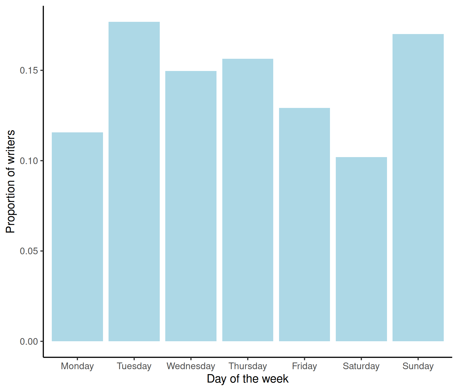

As our count data showed, there isn’t a great difference in the proportion of people born on any given day of the week, but it’s always useful to make a nice visualisation!

Calculating expected counts

What value would make sense for the expected count of Monday birthdays? Intuitively, it would make sense for the expected count of Monday birthdays, under the null hypothesis, would be 1/7 of all birthdays fall on a Monday.

Using the formula for the expected count, \(E_i = n \cdot p_{i,0}\), where \(n\) = sample size, \(p_{i,0}\) is the hypothesised population proportion for that category under the null hypothesis:

\[ 147 \cdot \frac{1}{7} = 21 \] We would expect the frequency of birthdays on a Monday to be 21.

To calculate our expected count for the other days of the week…

writers_table <- writers %>%
  group_by(DayOfWeek) %>%
  summarise(observed_count = n()) %>%
  mutate(expected_count = rep(147 * (1/7), 7))

writers_table

## # A tibble: 7 x 3
##   DayOfWeek observed_count expected_count
##   <fct>              <int>          <dbl>
## 1 Monday                17             21
## 2 Tuesday               26             21
## 3 Wednesday             22             21
## 4 Thursday              23             21
## 5 Friday                19             21
## 6 Saturday              15             21
## 7 Sunday                25             21

The rep(x, times) function will repeat x a given number of times.

Above, we calculated the expected count, 147 * (1/7) and then repeated it for the 7 days of the week. For this example, the null hypothesis specifies the same proportions for all 7 days of the week, hence the expected count for each day of the week is 21.

As we’ve calculated our expected count, we can also calculate our expected proportion. As there are 7 days of the week, we would expected the proportion of birthdays to fall equally across those days, i.e. 1/7 of birthdays fall on a Monday, 1/7 fall on a Tuesday etc.

writers_table <- writers %>%
 group_by(DayOfWeek) %>%
 summarise(observed_count = n()) %>%
 mutate(expected_count = rep(147 * (1/7), 7)) %>%
 mutate(expected_prop = rep(1/7, 7))

writers_table

## # A tibble: 7 x 4
##   DayOfWeek observed_count expected_count expected_prop
##   <fct>              <int>          <dbl>         <dbl>
## 1 Monday                17             21         0.143
## 2 Tuesday               26             21         0.143
## 3 Wednesday             22             21         0.143
## 4 Thursday              23             21         0.143
## 5 Friday                19             21         0.143
## 6 Saturday              15             21         0.143
## 7 Sunday                25             21         0.143

Performing the chi-square goodness-of-fit test

First, we need to calculate \(\frac{(O_i-E_i)^2}{E_i}\) for each day of the week (category).

writers_table <- writers_table %>%
  mutate(std_sq_diff = (observed_count - expected_count)^2 / expected_count)

writers_table

## # A tibble: 7 x 5
##   DayOfWeek observed_count expected_count expected_prop std_sq_diff
##   <fct>              <int>          <dbl>         <dbl>       <dbl>
## 1 Monday                17             21         0.143      0.762 
## 2 Tuesday               26             21         0.143      1.19  
## 3 Wednesday             22             21         0.143      0.0476
## 4 Thursday              23             21         0.143      0.190 
## 5 Friday                19             21         0.143      0.190 
## 6 Saturday              15             21         0.143      1.71  
## 7 Sunday                25             21         0.143      0.762

Standardised squared difference

How do we measure how far the observed counts are from the expected counts under the null? If we simply subtracted the expected counts from the observed counts and then add them up, you will get 0:

writers_diff <- writers_table$observed_count - writers_table$expected_count
sum(writers_diff)

## [1] 0

Instead, we will square the differences between the observed and expected counts, and then add them up.

One issue, however, remains to be solved. A squared difference between observed and expected counts of 100 has a different weight in these two scenarios:

Scenario 1: \(O = 30\) and \(E = 20\) leads to a squared difference \((O - E)^2 = 10^2 = 100\).

Scenario 2: \(O = 3000\) and \(E = 2990\) leads to a squared difference \((O - E)^2 = 10^2 = 100\)

However, it is clear that a squared difference of 100 in Scenario 1 is much more substantial than a squared difference of 100 in Scenario 2. It is for this reason that we divide the squared differences by the the expected counts to “standardize” the squared deviation.

The test-statistic \(\chi^2\) is obtained by adding up the standardized squared deviations and summing over all the categories.

Note: As \((O - E)^2\) is equal to \((E - O)^2\), the test-statistic can be written as:

\[ \chi^2 = \sum_i \frac{(O_i - E_i)^2}{E_i} = \sum_i \frac{(E_i - O_i)^2}{E_i} \]

Next, we need to sum our standard square differences column, to get out test statistic.

chi_stat <- sum(writers_table$std_sq_diff)
chi_stat

## [1] 4.857143

What does 4.85 mean?

If the observed and expected frequencies had been exactly equal, the chi-square statistic would have been 0 and you would have had no reason to doubt the null hypothesis that all days of the week are equally likely to be someone’s birthday.

\[ \chi^2 = \frac{(21 - 21)^2}{21} + \cdots + \frac{(21 - 21)^2}{21} = 0 \]

Large values of the test statistic constitute evidence against the null hypothesis. Answers will vary about whether this test statistic provides convincing evidence. We also need to calculate the p-value, using the pchisq function. You need to know how likely it is that you would obtain a test statistic this large (or larger) by random chance alone if all seven days of the week are equally likely to be a person’s birthday.

p-value

As always, your next step is to calculate the p-value.

The p-value tells you the probability of getting sample data at least as far from the hypothesized proportions as these data are, by random chance if the null hypothesis is true.

So again, a small p-value indicates the sample data is unlikely to have occurred by chance alone if the null hypothesis is true, providing evidence in favour of the alternative.

When the test statistic is large enough to produce a small p-value, then the sample data provide strong evidence against the null hypothesis

We will use the pchisq(<obs statistic>, df) function which wants our test statistic and degrees of freedom. Remember, our degrees of freedom are the # categories - 1, i.e. \(C - 1\).

1 - pchisq(chi_stat, df = 6)

## [1] 0.562262

If all seven days of the week are equally likely to be a person’s birthday, the probability that you would obtain a test statistic this large (or larger) by random chance alone is .56. With an \(\alpha = 0.05\), we fail to reject the null hypothesis that all seven days of the week are equally likely to be a person’s birthday, as the p-value (0.56)i s larger than the significance level.

Checking assumptions

Now for assumption checks:

1. Data should be randomly sampled from the population.
2. Data should be at the categorical or nominal level - goodness-of-fit test is not appropriate for continuous level data.
3. Expected counts should be at least 5.

Let’s check them:

1. Our data has not been randomly sampled from the population - these are the birthdays of “noted writers of the present” which is not a random sample of the population of all citizens.
2. Data is categorical (days of the week)
3. All expected counts were greater than 5 (expected birthdays for each day of the week was 21).

All in one function

As usual, R has a nifty function to calculate our test. The chisq.test() function requires x (the observed counts) and p (the expected proportions, a numerical vector):

gof_test <- chisq.test(x = writers_table$observed_count, 
                       p = writers_table$expected_prop)

gof_test

## 
##  Chi-squared test for given probabilities
## 
## data:  writers_table$observed_count
## X-squared = 4.8571, df = 6, p-value = 0.5623

The numbers all match!

Pearson residuals

If you were interested to know which day of the week had the highest contribution to the chi-square test statistic, you can calculate the Pearson residual.

# extracting the residuals from the performed chi square test performed above
gof_test$residuals 

## [1] -0.8728716  1.0910895  0.2182179  0.4364358 -0.4364358 -1.3093073  0.8728716

The highest values are for Tuesday and Saturday. The value for Tuesday, 1.09, is positive. This means that the observed counts were larger than expected. In the same way we interpret the residual for Saturday, -1.31. As this value is negative, this means that the observed counts of birthdays on a Saturday were less than expected.

Chi-square test of independence

The \(\chi^2\) test of independence is used to determine whether or not there is a significant association between two categorical variables.

Examples of when to use \(\chi^2\) test of independence

• We want to know if sex is associated with political party preference - we survey 1000 voters and record their sex and political party preference.

• If a person’s favourite colour is associated with their favourite sport - we survey 500 people and ask them about their preferences for both.

• Does telling a joke affect whether or not a waiter in a coffee sop receives a tip?

In each scenario we want to know if two categorical variables are associated with each other. We can use the \(\chi^2\) test of independence to determine if there is a statistically significant association between the variables.

Null hypothesis

\(H_0:\) Variable A is not associated with variable B

\(H_1:\) Variable A is associated with variable B

Test formula

\[ \chi^2 = \sum_{all\ cells} \frac{(O - E)^2}{E} \] where:

• \(\sum\) = the sum over all possible cells
• \(O\) = observed count for a cell
• \(E\) = expected count for a cell

If the p-value computed using a \(\chi^2\) distribution with (# rows - 1) \(\times\) (# columns - 1) is less than the chosen significance level (e.g. 0.05), then we can reject the null hypothesis.

Note that the formula is the same as the previous \(\chi^2\) test, but the degrees of freedom are different.

Assumptions

1. Two categorical variables

2. Two or more categories (groups) for each variable.

3. Independence of observations

• there is not relationship between the subjects in each group
• the categorical variables are not ‘paired’ in any way - e.g. pretest/post-test observations

4. Large enough sample size, such that:

• expected frequencies for each cell are at least 1
• expected frequencies should be at least 5 for the majority (80%) of cells

Checking assumptions

1. Study design issue - ensure that the data being collected are two categorical variables (not continuous or ordinal)
2. Study design issue
3. Study design issue - random sampling techniques help meet this assumption
4. Study design issue - ensure the study sample size is large enough before data collection

Question: Joking for a tip

Can telling a joke affect whether or not a waiter in a coffee bar receives a tip from a customer?

A study published in the Journal of Applied Social Psychology¹ investigated this question at a coffee bar of a famous seaside resort on the west Atlantic coast of France. The waiter randomly assigned coffee-ordering customers to one of three groups. When receiving the bill, one group also received a card telling a joke, another group received a card containing an advertisement for a local restaurant, and a third group received no card at all.

The data is stored in the file TipJoke.csv, accessible via the link https://uoepsy.github.io/data/TipJoke.csv. The variables are:

• Card: None, Joke, Ad.
• Tip: 1 = The customer left a tip, 0 = The customer did not leave tip.

In the following, we will consider leaving a tip as “success.”

Hypotheses

Question 1

Define the null and alternative hypothesis.

Solution

\(H_0:\) There is no association between card type and tipping.

\(H_1:\) The is an association between card type and tipping.

Question 2

Read in the data and run some checks.

Make sure the data is correctly encoded.

Solution

First we need to read in our data and see how it looks:

tipjoke <- read_csv('https://uoepsy.github.io/data/TipJoke.csv')

head(tipjoke) # print first 6 rows

## # A tibble: 6 x 2
##   Card    Tip
##   <chr> <dbl>
## 1 None      1
## 2 Joke      1
## 3 Ad        0
## 4 None      0
## 5 None      1
## 6 None      0

dim(tipjoke) # dimensions - 211 rows (observations) and 2 columns (variables)

## [1] 211   2

We need to make them both factors (as we’re working with categorical data) and change the Tip variable into NoTip and Tip to replace the 0s and 1s.

tipjoke <- tipjoke %>%
  mutate(Card = factor(Card),
         Tip = factor(Tip, levels = c(0, 1), labels = c('NoTip', 'Tip')))

head(tipjoke) # b-e-a-u-tiful

## # A tibble: 6 x 2
##   Card  Tip  
##   <fct> <fct>
## 1 None  Tip  
## 2 Joke  Tip  
## 3 Ad    NoTip
## 4 None  NoTip
## 5 None  Tip  
## 6 None  NoTip

Question 3

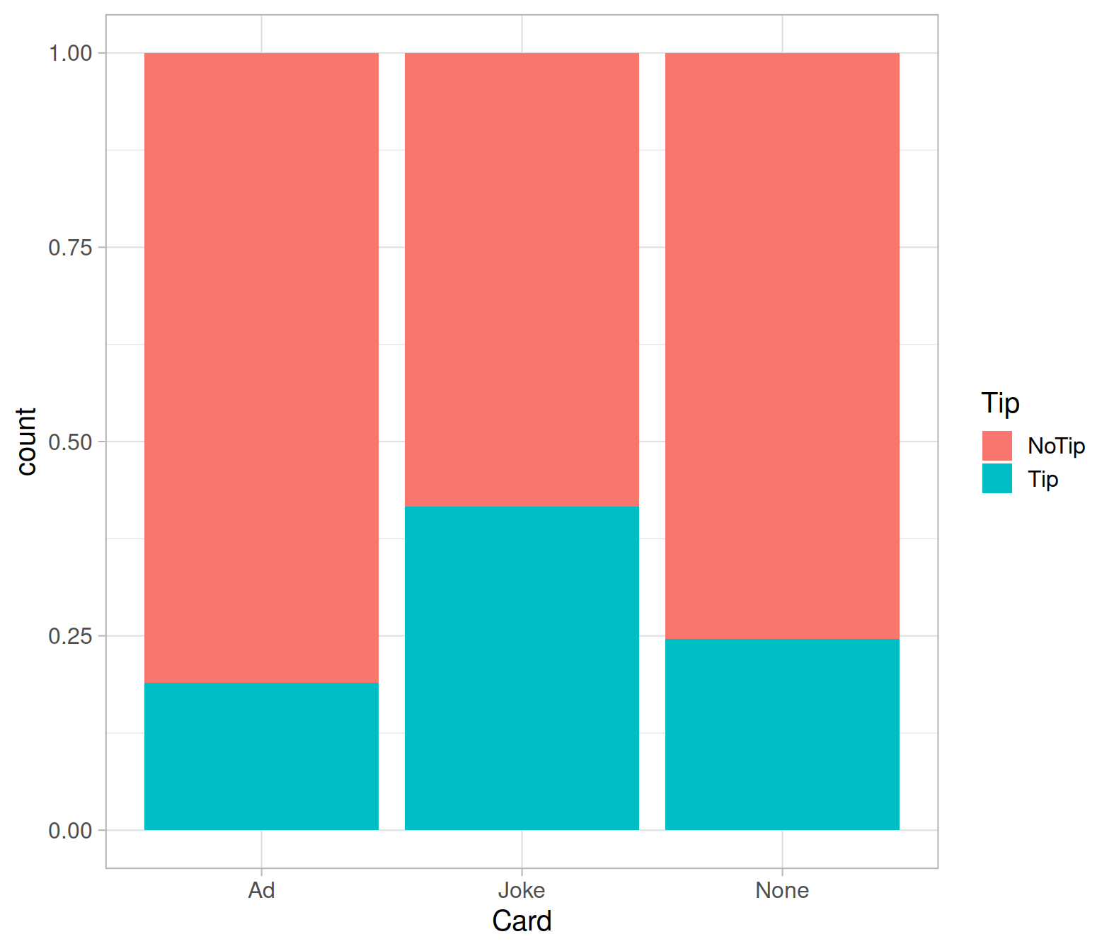
Create a barplot that visually summarises the data.

comment on what the graph shows.

Solution

ggplot(tipjoke, aes(x = Card, fill = Tip)) + # card on the x-axis and 'filling' the bar with our Tip variable (which has two levels)
  geom_bar()

From the stacked bar graph, it appears that perhaps the joke card does produce a higher success rate, but we need to investigate whether the differences are statistically significant.

If you prefer to have the bars all with the same heights and show the proportion of customers who tipped for each card, you can use:

ggplot(tipjoke, aes(x = Card, fill = Tip)) + 
  geom_bar(position = 'fill')

Question 4

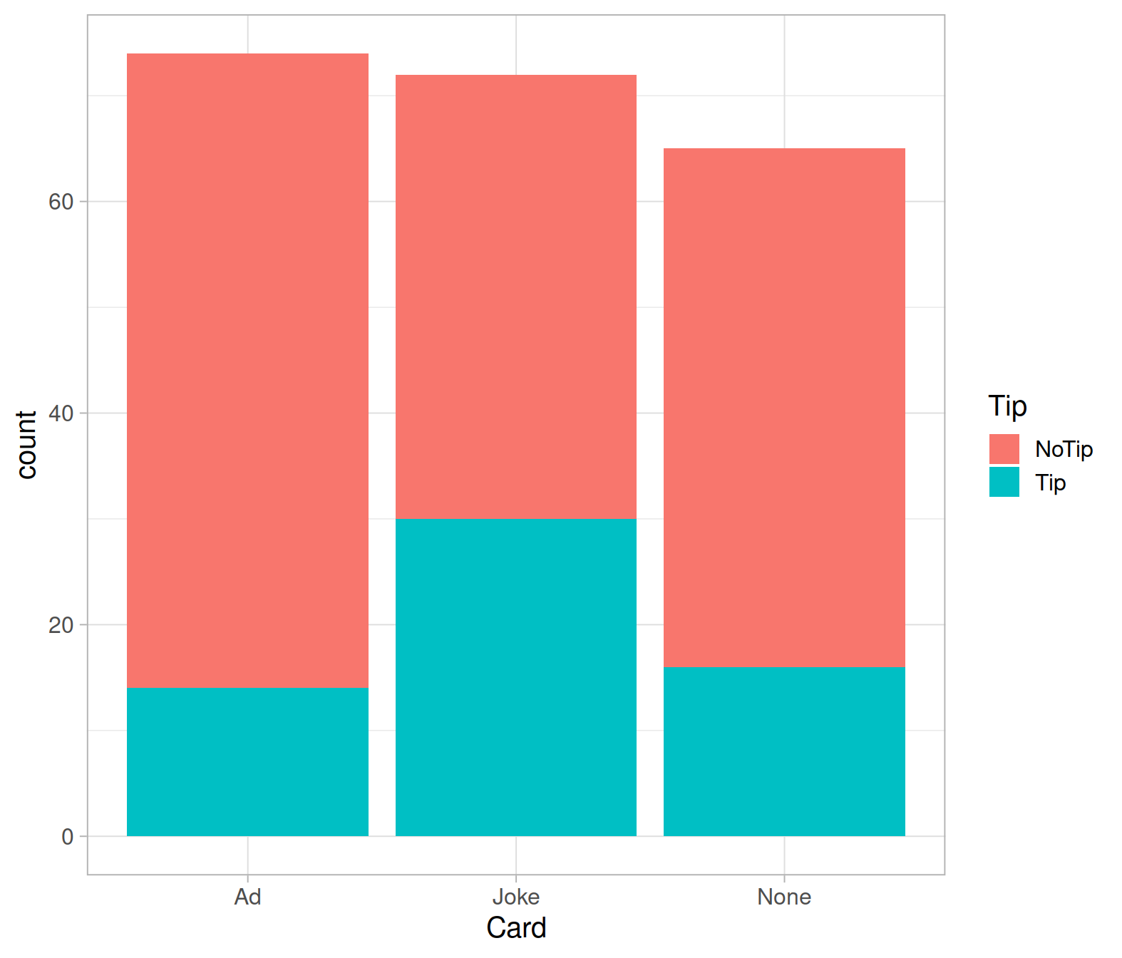
Create a two-way table showing how many customers left a tip or not, for each card type (including None).

Solution

observed_tipjoke <- table(tipjoke$Tip, tipjoke$Card)
observed_tipjoke

##        
##         Ad Joke None
##   NoTip 60   42   49
##   Tip   14   30   16

Question 5

Run a \(\chi^2\) test of independence, report the test statistic and the p-value.

Hint: For a test of independence, you need to provide to chisq.test() only one argument, x = the contingency table of observed counts

Solution

ind_test <- chisq.test(observed_tipjoke)
ind_test

## 
##  Pearson's Chi-squared test
## 
## data:  observed_tipjoke
## X-squared = 9.9533, df = 2, p-value = 0.006897

The \(\chi^2\) statistic in the sample is \(\chi^2\) = 9.95.

The p-value is \(P(\chi^2(2) \geq 9.95 = 0.007)\)

Question 6

Inspect the expected frequencies.

Look at the Pearson residuals and comment on what you notice.

Hint: look at the goodness-of-fit walkthrough and how we obtained the Pearson residuals - similar notation can be used to obtain the expected frequences too

Solution

ind_test$expected

##        
##               Ad     Joke     None
##   NoTip 52.95735 51.52607 46.51659
##   Tip   21.04265 20.47393 18.48341

ind_test$observed

##        
##         Ad Joke None
##   NoTip 60   42   49
##   Tip   14   30   16

More customers than expected under the null hypothesis:

• didn’t tip after receiving an advertising card;
• tipped after receiving a joke card;
• didn’t tip after receiving no card.

Less customers than expected under the null hypothesis:

• tipped after receiving an advertising card;
• didn’t tip after receiving a joke card;
• tipped after receiving no card.

ind_test$residuals

##        
##                 Ad       Joke       None
##   NoTip  0.9677724 -1.3270892  0.3641203
##   Tip   -1.5352747  2.1052950 -0.5776407

The top three contributions to the chi-square statistic are due to:

• more customers than expected under the null hypothesis tipped after receiving a joke card;
• less customers than expected under the null hypothesis tipped after receiving an advertisement card;
• less customers than expected under the null hypothesis didn’t tip after receiving a joke card.

Question 7

Check the assumptions of the test.

Solution

1. Data has two categorical variables (Card and Tip)
2. These categories had two and three groups for each variable (Card - 3 levels and Tip - 2 levels)
3. Independence of observations (a random sample was taken of a large population, no pairing)
4. Sample size was sufficiently large enough

• expected counts were all greater than 1
• and all cells had more than 5 expected counts

Question 8

Write a summary of the test results and relate back to the context of the study.

Solution

A \(\chi^2\) test of independence between tipping and card type was performed (\(\chi^2(2) = 9.95, p = .007\)). At the 5% significance level, the chi-square test indicates that there is very strong evidence that the tip rate differs depending on which card (Joke, Ad, or None) the waiter gave to the customer. In other words, the two variables are associated. To understand the nature of this difference in the chi-square test, we need to compare observed and expected frequencies. The observed number of tips in the joke group (30) is quite a bit higher than expected (20.47), while the observed counts for both the advertising and no card groups are lower than expected.

Glossary

• Cell contribution. The contribution of a cell in a table to the chi-square statistic. It is helpful in determining where large differences between observed data and what would be expected if the null hypothesis were true, exist.
• Chi-square statistic A standardized statistic for quantifying the distance between the observed frequencies in the sample with those expected under the null hypothesis.
• Observed counts. The observed frequencies in the cells of the table from the study.
• Expected counts. The expected frequencies for the cells of the table assuming the null hypothesis is true.
• Chi-square goodness-of-fit test. Are the proportions of the different categories in the population equal to the hypothesized proportions?
• Chi-square test of independence. Are two categorical variables independent in the population?

---

1. Gueaguen, N. (2002). The Effects of a Joke on Tipping When It Is Delivered at the Same Time as the Bill. Journal of Applied Social Psychology, 32(9), 1955-1963.↩︎