Hypothesis testing: the critical values approach

1. Recognise the difference between a bootstrap and null distribution
2. Understand the parallel between p-values and critical values
3. Be able to perform a one-sided or two-sided hypothesis test using the critical value method
4. Understand the link between z-scores and critical values

Research question and data

This week we will still be using the same data as last week, to see a direct comparison between the conclusions we reached using the p-value approach with the conclusions we will reach using the critical values approach.

Recall that the research question was:

Can a simple smile have an effect on punishment assigned following an infraction?

Data: Smiles.csv

Researchers LaFrance and Hecht (1995) conducted a study to examine the effect of a smile on the leniency of disciplinary action for wrongdoers. Participants in the experiment took on the role of members of a college disciplinary panel judging students accused of cheating. They were given, along with a description of the offence, a picture of the “suspect” who was either smiling or had a neutral facial expression. A leniency score (on a 10-point scale) was calculated based on the disciplinary decisions made by the participants. The full data can be found in the Smiles.csv dataset, also available at the following link: https://uoepsy.github.io/data/Smiles.csv

The experimenters have prior knowledge that smiling has a positive influence on people, and they are testing to see if the average lenience score is higher for smiling students than it is for students with a neutral facial expression (or, in other words, that smiling students are given more leniency and milder punishments.)

Analysing the data using a threshold of \(\alpha = 0.05\), last week we concluded that:

At a 5% significance level, we tested whether the mean leniency score for smiling students is higher than for students with a neutral expression. The p-value of the test (\(p = 0.029\)) indicates that if smiling truly had no effect on leniency scores, the chance of getting a difference in mean leniency scores between smiling and neutral students as high as 0.79 is 0.029, or 3 in 100 times. The sample data provide strong evidence against the null hypothesis that smiling had no effect on leniency and in favour of the alternative.

This week we will perform the same test of hypothesis, shown again below, but using the equivalent method of comparing the observed statistic with critical values. \[ H_0 : \mu_s - \mu_n = 0 \\ H_1 : \mu_s - \mu_n > 0 \]

Critical values

The critical values corresponding to a significance level of \(\alpha\) are the boundaries which delimit the regions leading to the rejection of the null hypothesis.

When the observed statistic is more extreme than the critical value, we reject the null hypothesis as such statistic would have a chance smaller than \(\alpha\) of occurring when \(H_0\) is true.

• The 95% critical value when \(H_1 : \mu > 0\) is found as the 95th percentile.

• The 95% critical values when \(H_1 : \mu \neq 0\) are two and are found as the 2.5th and 97.5th percentiles. The left critical value has a probability of 0.025 to its left, and the upper critical value has a probability of 0.025 to its right, which both sum to the desired 0.05.

First, we read the data into R and inspect the top six rows:

library(tidyverse)

smiles <- read_csv('https://uoepsy.github.io/data/Smiles.csv')
dim(smiles)

## [1] 68  2

We have 68 participants in the study and 2 variables. Let’s look at them:

head(smiles)

## # A tibble: 6 x 2
##   Leniency Group
##      <dbl> <chr>
## 1      7   smile
## 2      3   smile
## 3      6   smile
## 4      4.5 smile
## 5      3.5 smile
## 6      4   smile

Group is a categorical variable encoding which type of picture the panel was shown, either neutral or with a smile. It should be a factor:

smiles$Group <- as.factor(smiles$Group)
head(smiles)

## # A tibble: 6 x 2
##   Leniency Group
##      <dbl> <fct>
## 1      7   smile
## 2      3   smile
## 3      6   smile
## 4      4.5 smile
## 5      3.5 smile
## 6      4   smile

Let’s investigate the distribution of the original sample:

ggplot(smiles, aes(x = Leniency)) +
    geom_histogram(color = 'white', fill = 'lightblue', binwidth = 0.5) +
    facet_grid(Group ~ .)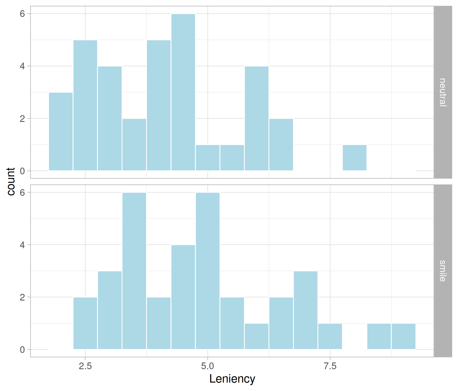

Before continuing, let’s compute the observed statistic in the sample:

stats <- smiles %>%
  group_by(Group) %>%
  summarise(Count = n(), 
            M = mean(Leniency), 
            SD = sd(Leniency))
stats

## # A tibble: 2 x 4
##   Group   Count     M    SD
##   <fct>   <int> <dbl> <dbl>
## 1 neutral    34  4.12  1.52
## 2 smile      34  4.91  1.68

Define

• \(\bar x_s\) = sample mean leniency score for smiling students
• \(\bar x_n\) = sample mean leniency score for students with a neutral expression

The observed statistic which estimates the population difference in means is: \[ \bar x_s - \bar x_n = 0.79 \]

The following code stores it in R:

D_obs <- diff(stats$M)
D_obs

## [1] 0.7941176

Null distribution: Resampling approach

The null distribution shows the possible values of a statistic for many samples from a population in which the null hypothesis is true.

First, we need to load the rep_randomize function:

source("https://uoepsy.github.io/files/rep_randomize.R")

For reproducibility, I will fix the random number generator seed, so that when I run again the entire file from start to finish I will get the same results.

set.seed(368)

Next, I will generate 1000 randomization samples. Each of such samples will be of size \(n = 68\) in which the group assignment has been shuffled.

rand_samples <- rep_randomize(smiles, columns = 'Group', samples = 1000)
rand_samples

## # A tibble: 68,000 x 3
##    sample Leniency Group  
##     <dbl>    <dbl> <fct>  
##  1      1      7   neutral
##  2      1      3   neutral
##  3      1      6   neutral
##  4      1      4.5 smile  
##  5      1      3.5 smile  
##  6      1      4   neutral
##  7      1      3   smile  
##  8      1      3   smile  
##  9      1      3.5 smile  
## 10      1      4.5 smile  
## # … with 67,990 more rows

The table above has 1,000 * 68 = 68,000 rows.

Then, for each randomization sample, we need to compute the difference in mean leniency score for the smiling and non-smiling students.

null_dist <- rand_samples %>%
  group_by(sample, Group) %>%
  summarise(M = mean(Leniency)) %>%
  group_by(sample) %>%
  summarise(D = diff(M))

null_dist

## # A tibble: 1,000 x 2
##    sample       D
##     <dbl>   <dbl>
##  1      1 -0.0588
##  2      2 -0.265 
##  3      3  0.0294
##  4      4 -0.265 
##  5      5 -0.0882
##  6      6 -0.0294
##  7      7 -0.265 
##  8      8  0.235 
##  9      9 -0.235 
## 10     10  0.294 
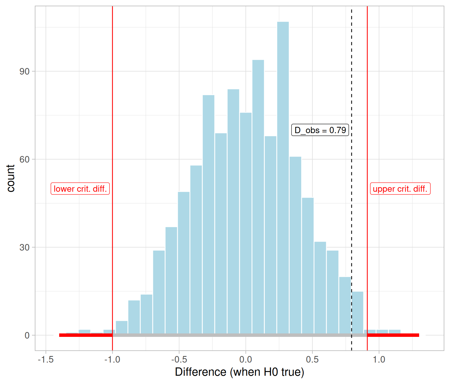
## # … with 990 more rows

We can visualise the null distribution of the difference in means and see where the observed difference falls in the distribution:

ggplot(null_dist, aes(x = D)) +
    geom_histogram(color = 'white', fill = 'lightblue') +
    geom_vline(xintercept = D_obs, color = 'black', linetype = 2) +
    annotate(geom = "label", x = D_obs, y = 70, label = 'D_obs = 0.79', 
             hjust = -0.05, size = 4, color = 'black', fill = 'white') +
    labs(x = "Difference (when H0 true)")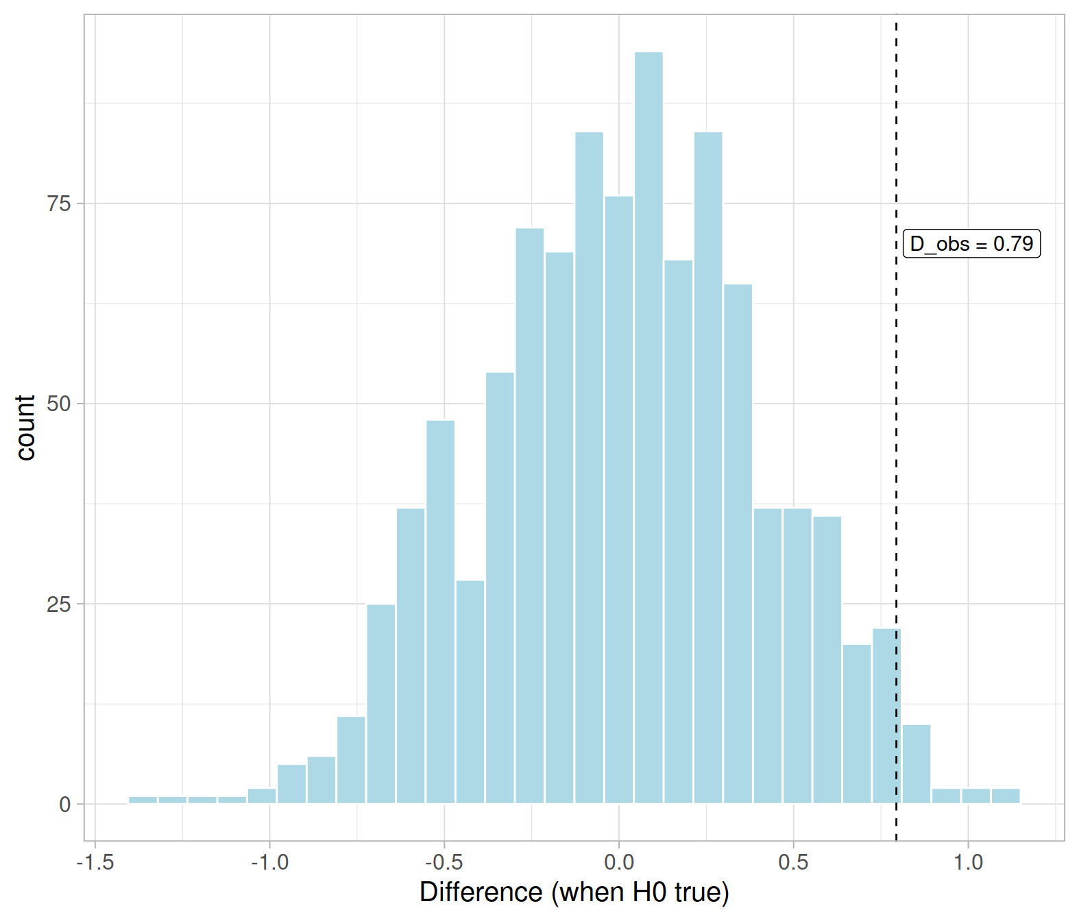

In the code above, linetype = 2 tells R to use a dashed line. Possible other values are 1 = solid line, 3 = dotted, 4 = dash-dotted line.

Don’t worry about annotate yet. It is used to make a pretty annotation at x = 0.79 and height y = 70 to not interfere with the rest of the graph (you can pick any other height you wish). The text to write is provided in label, while size controls the font size, color the colour, and fill the label fill colour. The argument hjust is the horizontal adjustment of the text, and can range from 0 to 1.

We now need to divide the x-axis (Differences when H0 is true) into two intervals:

• one leading to the rejection of \(H_0\)
• the other meaning that we do not have sufficient evidence to reject \(H_0\), i.e. the non-rejection region.

First, we need to specify the significance level, i.e. the proportion of statistics from the null distribution we don’t mind sacrificing and saying H0 is false (even if they came from H0) because they are sufficiently extreme.

Today, we will use \(\alpha = 0.05\), as statistics that only occur 5 in 100 times under the null are rare enough for this application.

Next, we need to find the critical difference that cuts an area of 0.95 to its left and 0.05 to its right:

D_crit <- quantile(null_dist$D, probs = 0.95)
D_crit

##       95% 
## 0.6764706

The critical difference, i.e. the 95th quantile of the null distribution, divides the possible values for the differences into two intervals

• Non-rejection region (NRR), going from \(-\infty\) to 0.68
• Rejection Region (RR), going from 0.68 to \(\infty\)

The following code displays the rejection region as a red horizontal line and the non-rejection region as a grey horizontal line:

ggplot(null_dist, aes(x = D)) +
    geom_histogram(color = 'white', fill = 'lightblue') +
    geom_segment(aes(x = D_crit, xend = 1.3, y = 0, yend = 0), 
                 color = 'red', size = 2) +
    geom_segment(aes(x = -1.4, xend = D_crit, y = 0, yend = 0), 
                 color = 'gray', size = 2) +
    geom_vline(xintercept = D_obs, color = 'black', linetype = 2) +
    geom_vline(xintercept = D_crit, color = 'red') +
    annotate(geom = "label", x = D_obs, y = 70, label = 'D_obs = 0.79', 
             size = 4, color = 'black', fill = 'white', hjust = -0.05) +
    annotate(geom = "label", x = D_crit, y = 50, label = 'D_crit = 0.68', 
             size = 4, color = 'red', fill = 'white', hjust = -0.05) +
    labs(x = "Difference (when H0 true)")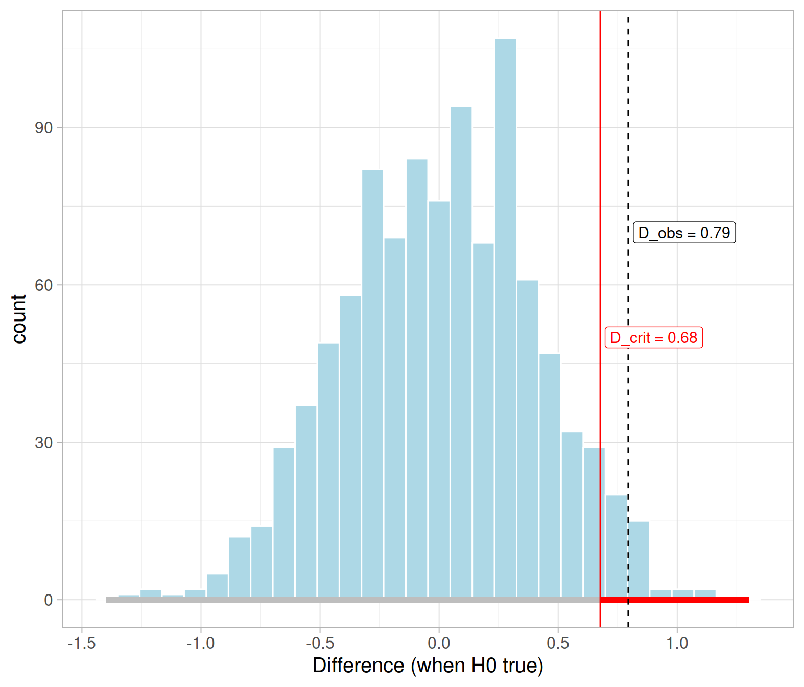

You see highlighted in red on the horizontal axis the differences that are more extreme than the critical value, and if the observed difference falls into that red region (the rejection region) our conclusion would be to reject the null hypothesis.

The grey region, instead, denotes the non-rejection region. If your observed difference falls into this grey part, you wouldn’t reject the null.

In our case,

At the 5% significance level, we tested whether smiling leads, on average, to more leniency compared to non-smiling. The observed difference in leniency means for smiling and non-smiling students is 0.79, which is larger than the critical difference 0.68 cutting a probability of 0.05 to its right. Hence, the sample difference in leniency means provides evidence against the null and in favour of the hypothesis that smiling does, on average, increase leniency and result in milder punishments.

Null distribution: Theoretical approach

We know from theory that the difference in means, when there is no difference in the population in mean leniency scores between smiling and non-smiling (i.e. when \(H_0 : \mu_s - \mu_n = 0\) is true), is \[ \bar X_s - \bar X_n \sim N(0, SE), \qquad \qquad SE = \sqrt{\frac{s_s^2}{n_s} + \frac{s_n^2}{n_n}} \] where \(s_s\) and \(s_n\) are the standard deviation of leniency for smiling and non-smiling students, respectively, in the original data.

Recall that we already computed the summary statistics for our data:

stats

## # A tibble: 2 x 4
##   Group   Count     M    SD
##   <fct>   <int> <dbl> <dbl>
## 1 neutral    34  4.12  1.52
## 2 smile      34  4.91  1.68

mu_theory <- 0

se_theory <- sqrt(stats$SD[1]^2 / stats$Count[1] + stats$SD[2]^2 / stats$Count[2])
se_theory

## [1] 0.38898

Let’s compare this with the standard error computed before via randomization, which was 0.4. As we can see they nicely agree!

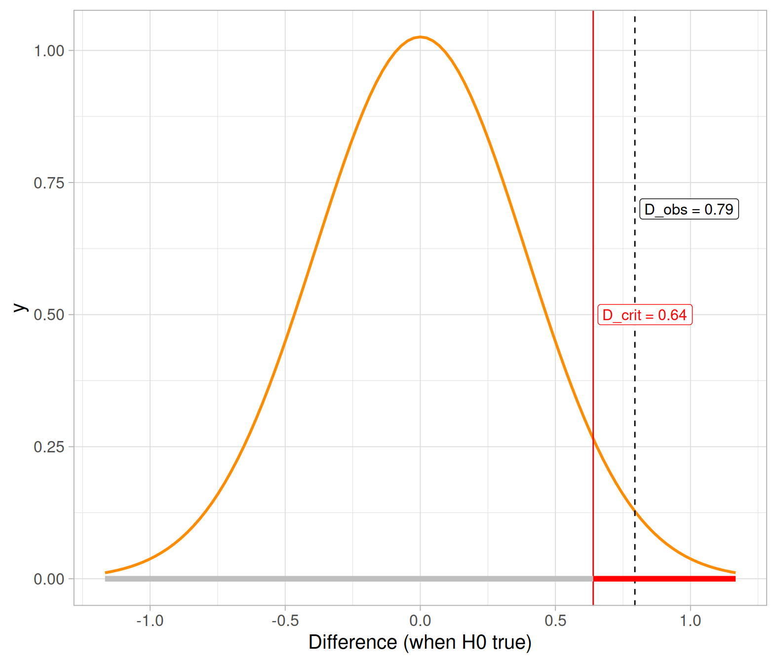
We now need to find the critical value that cuts a probability of 0.95 to its left (and 0.05 to its right):

D_crit_theory <- qnorm(p = 0.95, mean = mu_theory, sd = se_theory)
D_crit_theory

## [1] 0.6398152

Is the observed difference in means larger than the critical difference?

D_obs >= D_crit_theory

## [1] TRUE

This shows how the theory-based approach would lead to the same conclusion. At the 5% significance level, you would reject the null hypothesis.

Let’s also visualise this:

Exercises

Imagine now the scenario where the researchers have no prior beliefs about the effect of smiling on leniency scores, and they are testing to see if facial expression has any effect (it could either increase or decrease leniency scores if a disciplinary panel will view smiling as arrogant and disrespectful).

Question 1

State what the null and alternative hypothesis would have been in this scenario.

Solution

We are testing to see if there is evidence that the average score for smiling students is less than the average score for neutral students, so the alternative hypothesis is \(\mu_s < \mu_n\).

The null hypothesis is still “no effect”: \[ H_0 : \mu_s = \mu_n \\ H_1 : \mu_s < \mu_n \]

or, equivalently: \[ H_0 : \mu_s - \mu_n = 0 \\ H_1 : \mu_s - \mu_n < 0 \]

Question 2

Conduct a test of hypothesis at the \(\alpha = 0.01\) significance level using the critical value method.

Hints

1. Remember, you can reuse the null distribution we created above!

2. Find the correct quantiles

3. Check whether the observed difference falls in the non-rejection region

Solution

If the “red” area in the two tails must sum to 0.01, there will be a probability of \(0.01 / 2 = 0.005\) in each tail.

Hence, the required percentiles are the 0.5th and 99.5th percentiles. That is, we need to find (a) the quantile that has a probability of 0.005 to its left, and (b) the quantile that has a probability of 0.995 to its left and 0.005 to its right:

D_crits <- quantile(null_dist$D, probs = c(0.005, 0.995))
D_crits

##       0.5%      99.5% 
## -1.0002941  0.9119118

The non-rejection region will be the interval from -1 to 0.91.

Let’s check whether the observed difference falls within the non-rejection region:

D_obs

## [1] 0.7941176

The observed difference in means of 0.79 falls within the interval containing 99% of the values in the null distribution of the differences. Hence, a difference that big is deemed plausible to occur under the null hypothesis and at the 1% significance level, the observed difference does not provide sufficient evidence to reject the null hypothesis that the mean leniency for smiling students is different than for non-smiling students.

Question 3

Theoretical approach

You could perform the two-sided test of hypothesis above without the need for any resampling. To do so, you just need to original sample data and the theoretical formula, which is recalled below for convenience:

\[ \text{When }H_0\text{ is true:} \qquad \bar X_s - \bar X_n \sim N(0, SE), \qquad SE = \sqrt{\frac{s_s^2}{n_s} + \frac{s_n^2}{n_n}} \]

Conduct a test of hypothesis for the two-sided alternative using \(\alpha = 0.01\), the critical value approach, and resort to the theoretical distributions.

Solution

We know that if the null hypothesis is true, the difference in means is ditributed as a normal with zero mean and standard error:

se_theory <- sqrt(stats$SD[1]^2 / stats$Count[1] + stats$SD[2]^2 / stats$Count[2])

The 0.005 and 0.995 quantiles for such normal distribution are:

D_crits_theory <- qnorm(p = c(0.005, 0.995), mean = 0, sd = se_theory)
D_crits_theory

## [1] -1.001946  1.001946

We have a non-rejection region going from -1 to 1.

The observed difference in means is

D_obs

## [1] 0.7941176

At the 1% significance level, we conducted a two-sided test against the null hypothesis that the mean leniency score is the same for all smiling and non-smiling students. The observed difference of 0.79 falls within the 0.5th and 99.5th percentiles of the distribution, meaning that, at the 1% significance level, the observed difference doesn’t provide sufficient evidence against the null hypothesis.

Question 4

Theoretical approach: Standardization

We know that standardization makes data have a mean of 0 and standard deviation equal to 1. Furthermore we also know that for bell-shaped distributions, 95% of the values are between the mean - 1.96 * SD and the mean + 1.96 * SD.

For standardized variables, 95% of the values will be between -1.96 and 1.96, because mean = 0 and SD = 1.

\[ \text{When } H_0 \text{ is true:} \qquad \frac{(\bar X_s - \bar X_n) - 0}{SE} \sim N(0, 1) \] Using the standard normal distribution, check whether the observed difference falls into the rejection region of the distribution at the 5% significance level.

Solution

z_obs <- (D_obs - 0) / se_theory
z_obs

## [1] 2.041538

Let’s check that the relevant quantiles are -1.96 and 1.96:

qnorm(p = c(0.025, 0.975), mean = 0, sd = 1)

## [1] -1.959964  1.959964

At the 5% significance level, the observed standardized difference in means (2.04) is larger than the upper standardized critical difference in means (1.96). This leads us to reject the null hypothesis.

WARNING

Do not change the significance level throughout your analysis. These exercises are made for you to practice with multiple scenarios, but you should state and fix your significance level \(\alpha\) at the start of your research project and keep it the same throughout. Adjusting the significance level so that your results become significant is not good scientific practice.

Question 5

Theoretical approach: Another view

We have seen before that \[ \text{When }H_0\text{ is true:} \qquad \bar X_s - \bar X_n \sim N(0, SE), \qquad SE = \sqrt{\frac{s_s^2}{n_s} + \frac{s_n^2}{n_n}} \]

We also know that for bell-shaped distributions such as the normal, 95% of the values are between the mean - 1.96 * SD and the mean + 1.96 * SD.

In this case, 95% of the sample differences will be between \(-1.96 \cdot SE\) and \(1.96 \cdot SE\).

If we allocate a 5% significance level to the tails of the distribution, -1.96 and 1.96 will be our critical values. So we would reject whenever the observed difference in means \(\bar x_s - \bar x_n\) is larger, in absolute value, than 1.96 * SE:

\[ \text{Reject }H_0\text{ if:} \qquad | \bar x_s - \bar x_n | \geq 1.96 \cdot SE \]

Use the following quick rule to see if it leads to the same conclusions reached previously.

Solution

Recall the SE is computed as:

se_theory <- sqrt(stats$SD[1]^2 / stats$Count[1] + stats$SD[2]^2 / stats$Count[2])
se_theory

## [1] 0.38898

Check whether the observed difference is either

• larger than the hypothesised value + 1.96 * SE
• or smaller than the hypothesised value - 1.96 * SE

D_obs >= 1.96 * se_theory

## [1] TRUE

D_obs <= -1.96 * se_theory

## [1] FALSE

Alternatively, we can make the observed difference always positive by taking the absolute value, which drops any negative sign:

abs(D_obs) >= 1.96 * se_theory

## [1] TRUE

Hence, we reject the null hypothesis.

References

LaFrance, Marianne, and Marvin A Hecht. 1995. “Why Smiles Generate Leniency.” Personality and Social Psychology Bulletin 21 (3): 207–14.