Collecting data
PRE-LAB ACTIVITIES
Please ensure you have successfully installed R and RStudio, or are working on RStudio Cloud, and that you have completed the tasks on the Getting started in R & RStudio page, which introduced the basics of a) how to navigate around Rstudio, b) how to create a Rmarkdown document, c) how to read data into R, and d) how to use R to do basic arithmetic.
LEARNING OBJECTIVES
- Understand the link between study design and data we analyse.
- Understand and define different types of data.
- Understand and define data types with psychological examples.
In this lab, we are going to take a look at how to access specific sections of data, before we move on to talking about different types of data.
We encourage you to work along with the reading - open a new RMarkdown document, and run the code which we discuss below.
At the end there is a set of exercises for you to complete.
Accessing parts of the data
Suppose we read some data into R:
library(tidyverse)
starwars2 <- read_csv("https://uoepsy.github.io/data/starwars2.csv")
Reading data from a URL
Note that when you have a url for some data, such as https://uoepsy.github.io/data/starwars2.csv, you can read it in directly by giving functions like read_csv() the url inside quotation marks.
The data contains information on various characteristics of characters from Star Wars. We can print out the top of the data by using the name we just gave it:
starwars2## # A tibble: 75 x 6
## name height hair_color eye_color homeworld species
## <chr> <dbl> <chr> <chr> <chr> <chr>
## 1 Luke Skywalker 172 blond blue Tatooine Human
## 2 C-3PO 167 <NA> yellow Tatooine Human
## 3 R2-D2 96 <NA> red Naboo Droid
## 4 Darth Vader 202 none yellow Tatooine Human
## 5 Leia Organa 150 brown brown Alderaan Human
## 6 Owen Lars 178 brown, grey blue Tatooine Human
## 7 Beru Whitesun lars 165 brown blue Tatooine Human
## 8 R5-D4 97 <NA> red Tatooine Droid
## 9 Biggs Darklighter 183 black brown Tatooine Human
## 10 Obi-Wan Kenobi 182 auburn, white blue-gray Stewjon Human
## # … with 65 more rowsAlternatively, you could use the head() function which displays the first six rows of the data by default. You could change this by saying, for example, head(data, n = 10):
head(starwars2)## # A tibble: 6 x 6
## name height hair_color eye_color homeworld species
## <chr> <dbl> <chr> <chr> <chr> <chr>
## 1 Luke Skywalker 172 blond blue Tatooine Human
## 2 C-3PO 167 <NA> yellow Tatooine Human
## 3 R2-D2 96 <NA> red Naboo Droid
## 4 Darth Vader 202 none yellow Tatooine Human
## 5 Leia Organa 150 brown brown Alderaan Human
## 6 Owen Lars 178 brown, grey blue Tatooine Human(Don’t worry about the
Tip: Try clicking on the data in your environment (the top right window of RStudio). It will open the data in a tab in the editor window - this is another way of looking at the data, more like you would in spreadsheet software like Microsoft Excel. This can be time-consuming if your data file is big.
We can take a look at how big the data is (the dimensions), using dim()
dim(starwars2)## [1] 75 6There’s a reasonable amount of data in there - 75 rows and 6 columns.
In the starwars2 data, each character is an observational unit, and there are 6 variables (things which vary between units) such as their height, species, homeworld, etc.
Units and variables
The individual entities on which data are collected are called observational units or cases. Often (but not always), these equate to the rows of a dataset.
A variable is any characteristic that varies from observational unit to observational unit (these are often the columns of the dataset)
What if we want to extract certain subsections of our dataset, such as specific observational units or variables?
This is where we learn about two important bits of R code used to access parts of data - the dollar sign $, and the square brackets [].
The dollar sign $
The dollar sign allows us to extract a specific variable from a dataframe.
For instance, we can pull out the variable named “eye_color” in the data, by using $eye_color after the name that we gave our dataframe:
starwars2$eye_color## [1] "blue" "yellow" "red" "yellow"
## [5] "brown" "blue" "blue" "red"
## [9] "brown" "blue-gray" "blue" "blue"
## [13] "blue" "brown" "black" "orange"
## [17] "hazel" "blue" "yellow" "brown"
## [21] "red" "brown" "blue" "orange"
## [25] "blue" "brown" "black" "red"
## [29] "blue" "orange" "orange" "orange"
## [33] "yellow" "orange" NA "brown"
## [37] "yellow" "pink" "hazel" "yellow"
## [41] "black" "orange" "brown" "yellow"
## [45] "black" "brown" "blue" "orange"
## [49] "yellow" "black" "blue" "brown"
## [53] "brown" "blue" "yellow" "blue"
## [57] "blue" "brown" "brown" "brown"
## [61] "brown" "yellow" "yellow" "black"
## [65] "black" "blue" "unknown" "unknown"
## [69] "gold" "black" "green, yellow" "blue"
## [73] "brown" "black" NAEach variable in a dataframe is a vector. Once extracted, we will have a vector and not a dataframe.
The square brackets []
Square brackets are used to do what is known as indexing (finding specific entries in your data).
We can retrieve bits of data by identifying the \(i^{th}\) entry(s) inside the square brackets, for instance:
# assign the numbers 10, 20 ... 100 to the name "somevalues"
somevalues <- c(10, 20, 30, 40, 50, 60, 70, 80, 90, 100)

# pull out the 3rd entry
somevalues[3]
## [1] 30In a dataframe we have an extra dimension - we have rows and columns. Using square brackets with a dataframe needs us to specify both:
Let’s look at some examples:
# first row, fourth column:
starwars2[1, 4]
## # A tibble: 1 x 1
## eye_color
## <chr>
## 1 blue# tenth row, first column:
starwars2[10, 1]## # A tibble: 1 x 1
## name
## <chr>
## 1 Obi-Wan KenobiIf we leave either rows or columns blank, then we will get out all of them:
# tenth row, all columns:
starwars2[10, ]
## # A tibble: 1 x 6
## name height hair_color eye_color homeworld species
## <chr> <dbl> <chr> <chr> <chr> <chr>
## 1 Obi-Wan Kenobi 182 auburn, white blue-gray Stewjon Human# all rows, 2nd column:
starwars2[ , 2]## # A tibble: 75 x 1
## height
## <dbl>
## 1 172
## 2 167
## 3 96
## 4 202
## 5 150
## 6 178
## 7 165
## 8 97
## 9 183
## 10 182
## # … with 65 more rowsThere are is another way to identify column - we can use the name in quotation marks:
# first row, "species" column
starwars2[1, "species"]
## # A tibble: 1 x 1
## species
## <chr>
## 1 Human
Finally, we can also ask for multiple rows, or multiple columns, or both! To do that, we use the combine function c():
# the 1st AND the 6th row,
# and the 1st AND 3rd columns:
starwars2[c(1,6), c(1,3)]
## # A tibble: 2 x 2
## name hair_color
## <chr> <chr>
## 1 Luke Skywalker blond
## 2 Owen Lars brown, grey
And we can specify a sequence using the colon, from:to:
# FROM the 1st TO the 6th row, all columns:
starwars2[1:6, ]
## # A tibble: 6 x 6
## name height hair_color eye_color homeworld species
## <chr> <dbl> <chr> <chr> <chr> <chr>
## 1 Luke Skywalker 172 blond blue Tatooine Human
## 2 C-3PO 167 <NA> yellow Tatooine Human
## 3 R2-D2 96 <NA> red Naboo Droid
## 4 Darth Vader 202 none yellow Tatooine Human
## 5 Leia Organa 150 brown brown Alderaan Human
## 6 Owen Lars 178 brown, grey blue Tatooine HumanWhy? Because the colon operator, from:to, creates a vector from the value from to the value to in steps of 1.
1:6## [1] 1 2 3 4 5 6
The dollar sign $
Used to extract a variable from a dataframe:
dataframe$variable
The square brackets []
Used to extract parts of an R object by identifying rows and/or columns, or more generally, “entries.” Left blank will return all.
vector[entries]dataframe[rows, columns]
Accessing by a condition
We can also do something really useful, which is to access all the entries in the data for which a specific condition is true.
Let’s take a simple example to start:
somevalues <- c(10, 10, 0, 20, 15, 40, 10, 40, 50, 35)To only select values which are greater than 20, we can use:
somevalues[somevalues > 20]## [1] 40 40 50 35Let’s unpack what this is doing..
First, let’s look at what somevalues > 20 does. It returns TRUE for the entries of somevalues which are greater than 20, and FALSE for the entries of somevalues that are not (that is, which are less than, or equal to, 20.
This statement somevalues > 20 is called the condition.
somevalues > 20## [1] FALSE FALSE FALSE FALSE FALSE TRUE FALSE TRUE TRUE TRUEWe can give a name to this sequence of TRUEs and FALSEs
condition <- somevalues > 20
condition
## [1] FALSE FALSE FALSE FALSE FALSE TRUE FALSE TRUE TRUE TRUENow consider putting the sequence of TRUEs and FALSEs inside the square brackets in somevalues[].
This returns only the entries of somevalues for which the condition is TRUE.
somevalues[condition]## [1] 40 40 50 35So what we can do is use a condition inside the square brackets to return all the values for which that condition is TRUE.
Note that you don’t have to always give a name to the condition. This works too:
somevalues[somevalues > 20]## [1] 40 40 50 35
We can extend this same logic to a dataframe.
Let’s suppose we want to access all the entries in our Star Wars data who have the value “Droid” in the species variable.
To work out how to do this, we first need a line of code which defines our condition - one which returns TRUE for each entry of the species variable which is “Droid,” and FALSE for those that are not “Droid.”
We can use the dollar sign to pull out the species variable:
starwars2$species## [1] "Human" "Human" "Droid" "Human" "Human"
## [6] "Human" "Human" "Droid" "Human" "Human"
## [11] "Human" "Human" "Wookiee" "Human" "Rodian"
## [16] "Hutt" "Human" "Human" "Human" "Human"
## [21] "Trandoshan" "Human" "Human" "Mon Calamari" "Human"
## [26] "Ewok" "Sullustan" "Neimodian" "Human" "Gungan"
## [31] "Gungan" "Gungan" "Toydarian" "Dug" "unknown"
## [36] "Human" "Zabrak" "Twi'lek" "Twi'lek" "Vulptereen"
## [41] "Xexto" "Toong" "Human" "Cerean" "Nautolan"
## [46] "Zabrak" "Tholothian" "Iktotchi" "Quermian" "Kel Dor"
## [51] "Chagrian" "Human" "Human" "Human" "Geonosian"
## [56] "Mirialan" "Mirialan" "Human" "Human" "Human"
## [61] "Human" "Clawdite" "Besalisk" "Kaminoan" "Kaminoan"
## [66] "Human" "Aleena" "Skakoan" "Muun" "Togruta"
## [71] "Kaleesh" "Wookiee" "Human" "Pau'an" "unknown"And we can ask R whether each value is equal to “Droid” (Remember: in R, we ask whether something is equal to something else by using a double-equals, ==). A single equal sign would be wrong, as it denotes assignment.
starwars2$species == "Droid"## [1] FALSE FALSE TRUE FALSE FALSE FALSE FALSE TRUE FALSE FALSE FALSE FALSE
## [13] FALSE FALSE FALSE FALSE FALSE FALSE FALSE FALSE FALSE FALSE FALSE FALSE
## [25] FALSE FALSE FALSE FALSE FALSE FALSE FALSE FALSE FALSE FALSE FALSE FALSE
## [37] FALSE FALSE FALSE FALSE FALSE FALSE FALSE FALSE FALSE FALSE FALSE FALSE
## [49] FALSE FALSE FALSE FALSE FALSE FALSE FALSE FALSE FALSE FALSE FALSE FALSE
## [61] FALSE FALSE FALSE FALSE FALSE FALSE FALSE FALSE FALSE FALSE FALSE FALSE
## [73] FALSE FALSE FALSEFinally, we can use this condition inside our square brackets to access the entries of the data for which this condition is TRUE:
# I would read the code below as:

# "In the starwars2 dataframe, give me all the rows for which the
# condition starwars2$species=="Droid" is TRUE, and give me all the columns."

starwars2[starwars2$species == "Droid", ]
## # A tibble: 2 x 6
## name height hair_color eye_color homeworld species
## <chr> <dbl> <chr> <chr> <chr> <chr>
## 1 R2-D2 96 <NA> red Naboo Droid
## 2 R5-D4 97 <NA> red Tatooine Droid
Editing parts of the data
Now that we’ve seen a few ways of accessing sections of data, we can learn how to edit them!
Data Cleaning
One of the most common reasons you will need to modify entries in your data is in data cleaning. This is the process of identifying incorrect/incomplete/irrelevant data, and replacing/modifying/deleting them.
Changing specific entries
Above, we looked at the subsection of the data where the species variable had the entry “Droid.” Some of you may have noticed earlier that we had some data on C3PO. Is he not also a droid?

(Looks pretty Droid-y to me! disclaimer: I know nothing about Star Wars 🙂 )
Just as we saw above how to access specific entries, e.g.:
# 2nd row, all columns
starwars2[2, ]
## # A tibble: 1 x 6
## name height hair_color eye_color homeworld species
## <chr> <dbl> <chr> <chr> <chr> <chr>
## 1 C-3PO 167 <NA> yellow Tatooine Human# 2nd row, 6th column (the "species" column)
starwars2[2,6]## # A tibble: 1 x 1
## species
## <chr>
## 1 HumanWe can change these by assigning them a new value (remember the <- symbol):
# C3PO is a droid, not a human
starwars2[2,6] <- "Droid"

# Look at the 2nd row now -
# the entry in the "species" column has changed:
starwars2[2, ]
## # A tibble: 1 x 6
## name height hair_color eye_color homeworld species
## <chr> <dbl> <chr> <chr> <chr> <chr>
## 1 C-3PO 167 <NA> yellow Tatooine DroidThink of it as “overwriting,” “replacing,” or “reassigning”
We have replaced, or overwritten, the entry in the 2nd row and 6th column of the data (starwars2[2,6]) with the value “Droid.”
Changing entries via a condition
We saw above how to access parts of data by means of a condition, with code such as:
# "In the starwars2 dataframe, give me all the rows for which the
# condition starwars2$homeworld=="Naboo" is TRUE, and give me all the columns."

# remember, we're asking for all the columns by leaving it blank *after* the
# comma inside the square brackets: data[rows, columns]
starwars2[starwars2$homeworld=="Naboo", ]
## # A tibble: 8 x 6
## name height hair_color eye_color homeworld species
## <chr> <dbl> <chr> <chr> <chr> <chr>
## 1 R2-D2 96 <NA> red Naboo Droid
## 2 Palpatine 170 grey yellow Naboo Human
## 3 Jar Jar Binks 196 none orange Naboo Gungan
## 4 Roos Tarpals 224 none orange Naboo Gungan
## 5 Rugor Nass 206 none orange Naboo Gungan
## 6 Gregar Typho 185 black brown Naboo Human
## 7 Cordé 157 brown brown Naboo Human
## 8 Dormé 165 brown brown Naboo HumanWhat if we wanted to modify it so that every character from “Naboo” was actually of species “Nabooian?”
We can do that in a number of ways, all of which do the same thing - namely, they access parts of the data and assign them the new value “Nabooian.”
Study the lines of code below and their interpretations:
# In the starwars2 data, give the rows for which condition
# starwars2$homeworld=="Naboo" is TRUE, and select only the "species" column.
# Assign to these selected entries the value "Nabooian".
starwars2[starwars2$homeworld=="Naboo", "species"] <- "Nabooian"

# In the starwars2 data, give the rows for which condition
# starwars2$homeworld=="Naboo" is TRUE, and select only the 6th column.
# Assign to these selected entries the value "Nabooian".
starwars2[starwars2$homeworld=="Naboo", 6] <- "Nabooian"

# Extract the species variable from the starwars2 data (it's a vector).
# Pick the entries for which the condition starwars2$homeworld=="Naboo" is TRUE.
# Assign to these selected entries the value "Nabooian".
starwars2$species[starwars2$homeworld=="Naboo"] <- "Nabooian"
Changing a variable
Another thing we might want to do is change a whole variable (a whole column) in some way.
The logic is the same, for instance:
starwars2$height <- starwars2$height / 100What we have done above is taking the variable “height” from the dataframe “starwars2,” dividing it by 100 via starwars2$height / 100, and then assigning the result to the same variable, i.e. we overwrite the column.
Equally, we could also have added a new column named “height2” with those values if you do not want to overwrite “height”:
starwars2$height2 <- starwars2$height / 100This would have left the “height” variable as-is, and created a new one called “height2” which was the values in “height” divided by 100.
Removing rows or columns
Lastly, we might want to change the data by removing a row or a column.
Again, the logic remains the same, in that we use <- to assign the edited data to a name (either a new name, thus creating a new object, or an existing name, thereby overwriting that object).
For instance, notice that the 35th and 75th rows of our data probably aren’t a valid observation - I’m reasonably sure that Marge and Homer Simpson never appeared in Star Wars:
starwars2[c(35,75), ]## # A tibble: 2 x 6
## name height hair_color eye_color homeworld species
## <chr> <dbl> <chr> <chr> <chr> <chr>
## 1 Marge Simpson 1.7 Blue <NA> Springfield unknown
## 2 Homer Simpson 1.8 <NA> <NA> Springfield unknownWe can remove a certain row(s) by using a minus sign - inside the square brackets
# everything minus the 75th row
starwars2[-75, ]
## # A tibble: 74 x 6
## name height hair_color eye_color homeworld species
## <chr> <dbl> <chr> <chr> <chr> <chr>
## 1 Luke Skywalker 1.72 blond blue Tatooine Human
## 2 C-3PO 1.67 <NA> yellow Tatooine Droid
## 3 R2-D2 0.96 <NA> red Naboo Nabooian
## 4 Darth Vader 2.02 none yellow Tatooine Human
## 5 Leia Organa 1.5 brown brown Alderaan Human
## 6 Owen Lars 1.78 brown, grey blue Tatooine Human
## 7 Beru Whitesun lars 1.65 brown blue Tatooine Human
## 8 R5-D4 0.97 <NA> red Tatooine Droid
## 9 Biggs Darklighter 1.83 black brown Tatooine Human
## 10 Obi-Wan Kenobi 1.82 auburn, white blue-gray Stewjon Human
## # … with 64 more rows# everything minus the (35th and 75th rows)
starwars2[-c(35, 75), ]## # A tibble: 73 x 6
## name height hair_color eye_color homeworld species
## <chr> <dbl> <chr> <chr> <chr> <chr>
## 1 Luke Skywalker 1.72 blond blue Tatooine Human
## 2 C-3PO 1.67 <NA> yellow Tatooine Droid
## 3 R2-D2 0.96 <NA> red Naboo Nabooian
## 4 Darth Vader 2.02 none yellow Tatooine Human
## 5 Leia Organa 1.5 brown brown Alderaan Human
## 6 Owen Lars 1.78 brown, grey blue Tatooine Human
## 7 Beru Whitesun lars 1.65 brown blue Tatooine Human
## 8 R5-D4 0.97 <NA> red Tatooine Droid
## 9 Biggs Darklighter 1.83 black brown Tatooine Human
## 10 Obi-Wan Kenobi 1.82 auburn, white blue-gray Stewjon Human
## # … with 63 more rowsAnd we can simply re-use the name “starwars2” to overwrite the data and make this change take effect (rather than just print out the result, which the code above did):
starwars2 <- starwars2[-c(35, 75), ](now, in the environment pane of Rstudio, the object named “starwars2” will say 73 observations, rather than 75, which it had before - we’ve removed the 2 rows)
The same logic applies for columns:
# Create a new object called "anonymous_starwars2" and assign it
# to the values which are the "starwars2" dataframe minus the
# 1st column (the "name" column):
anonymous_starwars2 <- starwars2[, -1]

# print out anonymous_starwars2
anonymous_starwars2
## # A tibble: 73 x 5
## height hair_color eye_color homeworld species
## <dbl> <chr> <chr> <chr> <chr>
## 1 1.72 blond blue Tatooine Human
## 2 1.67 <NA> yellow Tatooine Droid
## 3 0.96 <NA> red Naboo Nabooian
## 4 2.02 none yellow Tatooine Human
## 5 1.5 brown brown Alderaan Human
## 6 1.78 brown, grey blue Tatooine Human
## 7 1.65 brown blue Tatooine Human
## 8 0.97 <NA> red Tatooine Droid
## 9 1.83 black brown Tatooine Human
## 10 1.82 auburn, white blue-gray Stewjon Human
## # … with 63 more rowsTypes of data
There are so many different things we can measure / record on observational units. Therefore the data we collect will also have different characteristics.
For instance, we could measure the colour of people’s hair as any of “black,” “brown,” “blond,” and so on, or we could use reflective spectrophotometry to obtain a number for the black/white-ness, a number for the red/green-ness, and a number for the blue/yellow-ness. One approach gives us a set of possible categories, the other gives us numbers. We distinguish between these different types in talking about categorical and numerical variables. Within each, there also are a few important sub-classes.
Categorical variables tell us what group or category each individual belongs to. Each distinct group or category is called a level of the variable.
| Type | Description | Example |
|---|---|---|
| Nominal (Unordered categorical) | A categorical variable with no intrinsic ordering among the levels. | Species: Human, Droid, Wookie, Hutt, … |
| Ordinal (Ordered categorical) | A categorical variable which levels possess some kind of order | Level: Low, Medium, High |
| Binary categorical | A special case of categorical variable with only 2 possible levels | Is_Human: Yes or No. |
Numerical (or quantitative) variables consist of numbers, and represent a measurable quantity. Operations like adding and averaging make sense only for numeric variables.
| Type | Description | Example |
|---|---|---|
| Continuous | Variables which can take any real number within the specified range of measurement | Height: 172, 165.2, 183, … |
| Discrete | Variables which can only take integer number values. For instance, a counts can only take positive integer values (0, 1, 2, 3, etc.) | Number_of_siblings: 0, 1, 2, 3, 4, … |
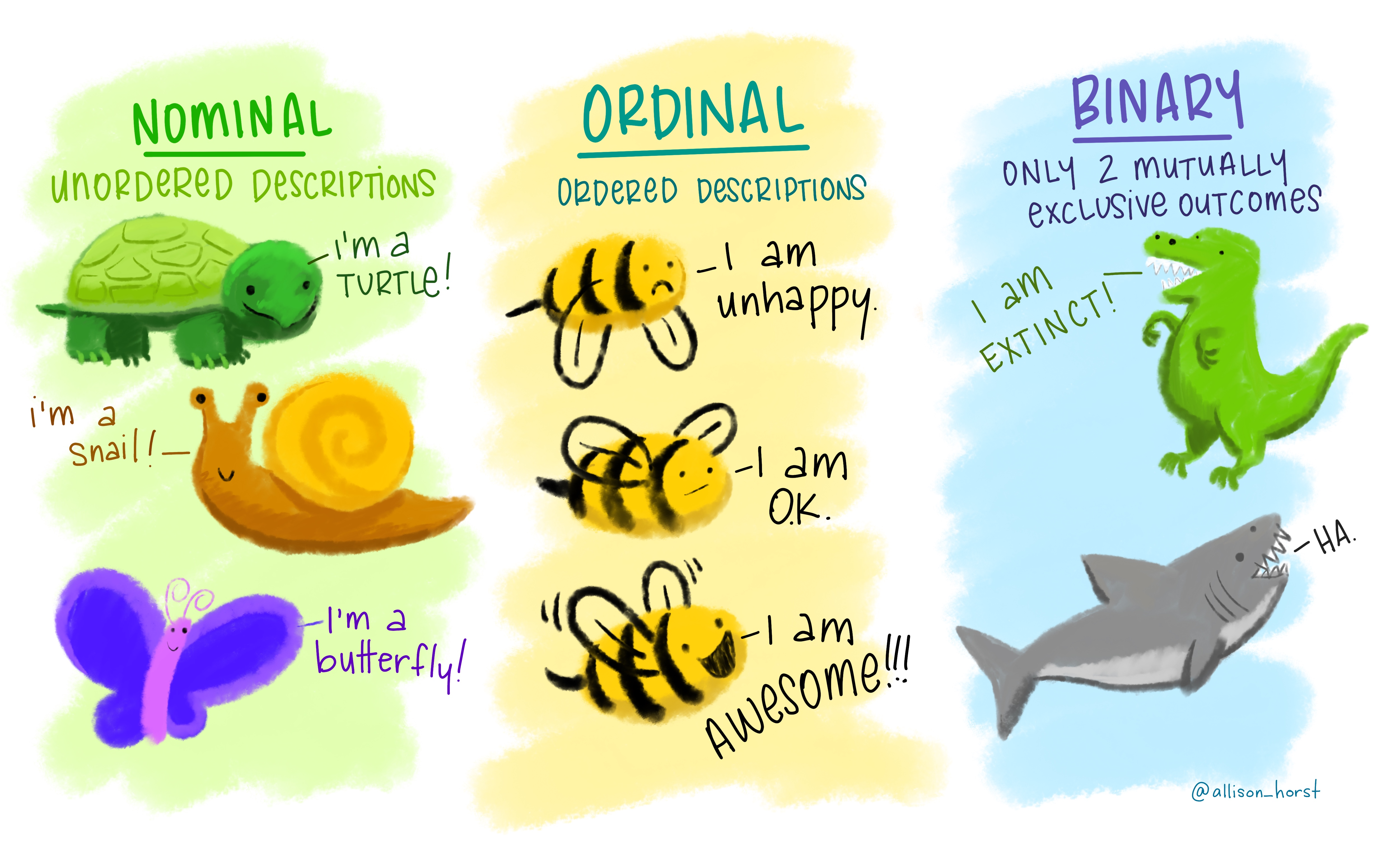
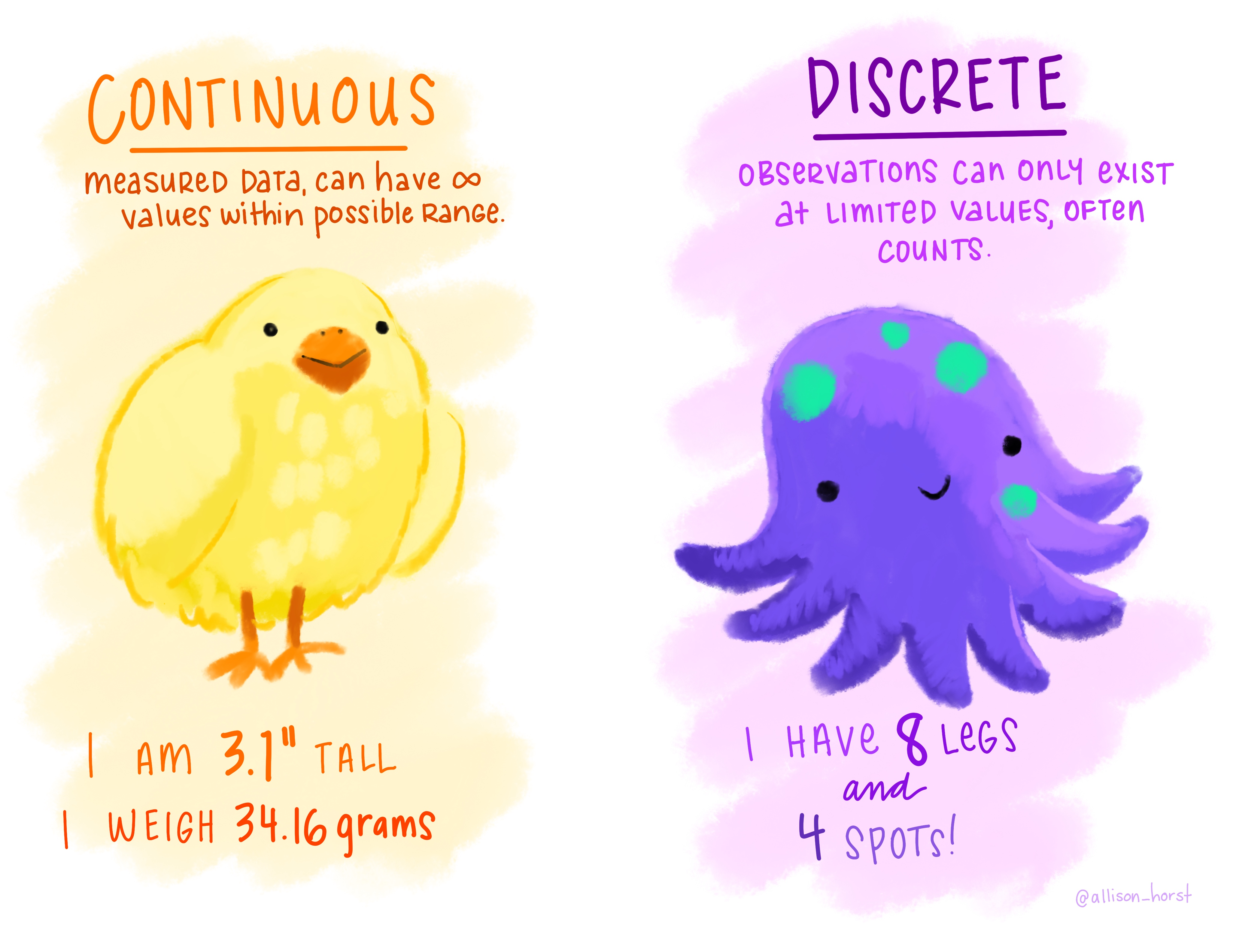
Figure 1: Artwork by @allison_horst
In R, different types of data get treated differently by functions, and we need to tell R explicitly what type of data each variable is.
Think about why we have to do this. All that data is, at its most fundamental level, is a set of symbols: e.g. “a,” “14,” etc. We need to tell R if our set of symbols “1,” “4,” “5” are numbers - and so can be added/subtracted etc - or if they correspond to categories. Alternatively, they might be neither, and just be a set of characters (symbols).
We can use some specific functions to both tell and ask R what type some data are:
| Type | Set as… | Check is… |
|---|---|---|
| Categorical | as.factor()factor() |
is.factor() |
| Ordered Categorical (Ordinal) | as.ordered()factor(... , ordered = TRUE) |
is.ordered() |
| Continuous | as.numeric() |
is.numeric() |
| Character | as.character() |
is.character() |
To check whether variables of a certain type, we can use these functions as follows:
is.character(starwars2$name)## [1] TRUEis.numeric(starwars2$height)## [1] TRUEis.factor(starwars2$species)## [1] FALSEAlternatively, we can also use the function class():
class(starwars2$height)## [1] "numeric"And we can modify the class of a variable by following the same syntax as we modified variables earlier, and using functions such as as.factor(), as.numeric():
# overwrite the "species" variable with a 'factorised' "species" variable:
starwars2$species <- as.factor(starwars2$species)
Check that it is now a factor:
class(starwars2$species)## [1] "factor"Factors have certain levels that values can take:
levels(starwars2$species)## [1] "Aleena" "Besalisk" "Cerean" "Chagrian" "Clawdite"
## [6] "Droid" "Dug" "Ewok" "Geonosian" "Human"
## [11] "Hutt" "Iktotchi" "Kaleesh" "Kaminoan" "Kel Dor"
## [16] "Mirialan" "Mon Calamari" "Muun" "Nabooian" "Nautolan"
## [21] "Neimodian" "Pau'an" "Quermian" "Rodian" "Skakoan"
## [26] "Sullustan" "Tholothian" "Togruta" "Toong" "Toydarian"
## [31] "Trandoshan" "Twi'lek" "Vulptereen" "Wookiee" "Xexto"
## [36] "Zabrak"Levels
In categorical data, each case has a value which is one of a fixed set of possibilities. The set of possibilities are the levels of a categorical variable.
If we were to try and set an entry as a value which is not one of those levels, it won’t work, and you’ll likely get an error such as:
# set the 1st row, 6th column (the species variable) to be "Peppapig"
starwars2[1, 6] <- "Peppapig"
invalid factor level, NA generated
Error: Assigned data "Peppapig" must be compatible with existing data.
One useful function which treats different classes of variable differently, is summary().
Notice how the output differs between variables such as height, which we know is numeric, species, which we just set to be categorical, and homeworld which is currently character (just text):
summary(starwars2)## name height hair_color eye_color
## Length:73 Min. :0.790 Length:73 Length:73
## Class :character 1st Qu.:1.670 Class :character Class :character
## Mode :character Median :1.800 Mode :character Mode :character
## Mean :1.762
## 3rd Qu.:1.910
## Max. :2.640
##
## homeworld species
## Length:73 Human :25
## Class :character Nabooian: 8
## Mode :character Droid : 2
## Kaminoan: 2
## Mirialan: 2
## Twi'lek : 2
## (Other) :32Glossary
- Data cleaning: The process of tidying data prior to analysis, e.g., removing impossible values.
- Condition: A (set of) properties which are either TRUE or FALSE for each datapoint.
- Categorical/qualitative variable: Data which has a discrete number of possible responses.
- Nominal: Data which has a discrete number of possible responses, without a natural ordering.
- Ordinal: Data which has a discrete number of possible responses, with a natural ordering, but the intervals between responses levels are unmeasurable.
- Binary: Data which has a two possible responses (e.g., TRUE/FALSE, YES/NO).
- Numerical/quantitative variable: Data which can take values on a numeric scale.
- Continuous variable: Data which can take values on a numeric scale and can take any real number within a range (e.g., 2.01, 2.009, 2.0099, …).
- Discrete variable: Data which can take only integer numeric values (no decimals). For example, count data can take only positive whole numbers: 0, 1, 2, 3, …
- character: In R, character variables can take any symbol (“a,” “9,”“1030394tkdjd,” …).
- numeric: In R, numeric variables can take any real number (-4, 0.5553, 105, …).
- factor: In R, factor variables can only take on categories from a specific set of allowed levels.
- level: Each distinct category that a factor variable can take in R.
[]and$for accessing and modifying entries within data stored in R.==“is equal to”!=“is not equal to”!“Not”<and<=“less than” and “less than or equal to”>and>=“greater than” and “greater than or equal to”is.factor(),is.numeric(),is.character(),is.ordered()to check whether a variable is coded as a specific type.class()for detemining what type a variable is coded as.as.factor()/factor(),as.numeric(),as.character(),as.ordered()to make a variable a specific type.levels()to see the possible response options of a factor (categorical) variablesummary()to see a summary of all variables in a dataframe (the summary is different for each variable depending on whether it is categorical/numeric).
Exercises
For the exercises, we have a dataset on some of the most popular internet passwords, their strength, and how long it took for an algorithm to crack it. The data is available online at https://uoepsy.github.io/data/passworddata.csv.
| Variable Name | Description |
|---|---|
| rank | Popularity in the database of released passwords |
| password | Password |
| type | Category of password |
| cracked | Time to crack by online guessing |
| strength | Strength = quality of password where 10 is highest, 1 is lowest |
| strength_cat | Strength category (weak, medium, strong) |
Open a new Rmarkdown document.
File > New File > R Markdown..
In your first code-chunk, load the tidyverse packages with the following command:
library(tidyverse)Make sure you run the chunk.
Read in the data from the link (https://uoepsy.github.io/data/passworddata.csv).
You may notice that the url ends with .csv. This means we can use the read_csv() function to read it into R.
Be sure to assign it a name, otherwise it will just print it out, and not store it in R’s environment!
Look at the 90th entry of the data, using the square brackets.
Show the 1st to 20th rows, and the password variable.
Is the type variable being treated as categorical by R? Check using the is.factor() function.
If it is not, then make it a factor.
What distinct levels does the type variable have?
Access all the data for passwords categorised as “fluffy,” and assign them to a new object called fluffy_passwords
What type do you think the strength_cat variable should be? Change it accordingly in the data.
Show all the data for passwords categorised as either “animal” or “sport.”
Note that this requires something which we didn’t mention above. In R, when you have multiple conditions (e.g, A and B, C or D), we can define them using:
&to mean “and”|to mean “or”
For instance, if we want to show the passwords which are
1. categorised as “fluffy”
AND
2. ranked in the top 50
# "In the pwords dataframe, give me all the rows for which the
# conditions pwords$type == "fluffy" AND pwords$rank <= 50 are TRUE,
# and give me all the columns."
pwords[(pwords$type == "fluffy") & (pwords$rank <= 50), ]
## # A tibble: 2 x 6
## rank password type cracked strength strength_cat
## <dbl> <chr> <fct> <dbl> <dbl> <ord>
## 1 42 love fluffy 7.92 6 medium
## 2 43 sunshine fluffy 6.91 9 medium
Finally, show all the data for which the passwords are not categorised as “fluffy.”
Recall from the introductory to R page, that in R we use an exclamation mark, !, to mean “not.”