Confidence Intervals & Bootstrapping

1. Understand how bootstrap resampling with replacement can be used to approximate a sampling distribution.
2. Understand how the bootstrap distribution can be used to construct a range of highly plausible values (a confidence interval).
3. Understand the link between simulation-based standard errors and theory-based standard errors.

Sampling distribution recap

• Instead of collecting data on an entire population, we often collect data on a sample drawn at random from that population.

• We can compute a statistic on our sample, which we can then use as an estimate of the equivalent parameter in the population.

  • For example, we can take a sample of 30 students and calculate their mean height (the sample statistic). This is our estimate of the mean height of all students (population parameter).

• However… sample statistics vary from sample to sample. Using a sample statistic as an estimate of a population parameter brings an element of uncertainty.

• By taking lots of samples and computing the statistic for each one, we can create a sampling distribution for that statistic. This allows us to quantify the variation in the sample statistics which is due to sampling.

• The standard deviation of the sampling distribution is known as the standard error.

• Finally, we saw how the size of our samples influences the sampling variation, with bigger samples leading to narrower sampling distributions, and more precise estimates.

Bootstrapping

In order to quantify the precision of our sample statistics as estimates of the population, we refer to the sampling distribution of the statistic.

Problem: in most real life research, we cannot observe the sampling distribution of a statistic. We have neither the time nor the resources to take many samples of size \(n\) in order to get an idea of how accurate an estimate is.
What can we do with only one sample?

Solution 1	Solution 2 (Bootstrapping)
Use the formula \(\text{SE} = \frac{\sigma}{\sqrt{n}}\), where \(\sigma\) is the standard deviation of the population, or our estimate of it (i.e., our sample standard deviation \(\hat \sigma\) or \(s\)), and \(n\) is our sample size.	Mimick the act of repeated sampling from the population by repeated resampling with replacement from the original sample.

Bootstrapping
Random sampling with replacement from the original sample, using the same sample size.

We can mimick the act of repeated sampling of \(n\) units from the population, by resampling with replacement \(n\) units from our original sample of \(n\) units.
When we resample with replacement from our original sample enough times, the distribution of resample statistics begins to approximate the sampling distribution of the sample statistic!.

Example: NFL Players

We are interested in the following question: what was the average yearly salary of a NFL player in 2015?

In this particular example, we are actually going to have access to data on the entire population, meaning that we will actually know the population parameter (the average yearly salary of NFL players in 2015). You can see these in the drop-down box below:

The population: NFL Players in 2015

We will read a file containing the yearly salaries (in millions of dollars) for all players being paid at the start of 2015 by a National Football League (NFL) team. This entire dataset represents the population of all National Football League players in 2015

nfl_pop <- read_csv("https://uoepsy.github.io/data/nflpop.csv")
head(nfl_pop)

## # A tibble: 6 x 5
##   Player             Position Team     TotalMoney YearlySalary
##   <chr>              <chr>    <chr>         <dbl>        <dbl>
## 1 Russell Wilson     QB       Seahawks        140         35  
## 2 Ben Roethlisberger QB       Steelers         68         34  
## 3 Aaron Rodgers      QB       Packers         134         33.5
## 4 Jared Goff         QB       Rams            134         33.5
## 5 Carson Wentz       QB       Eagles          128         32  
## 6 Matt Ryan          QB       Falcons         150         30

The population parameter:

nfl_pop %>% summarise(
  mean_salary = mean(YearlySalary)
)

## # A tibble: 1 x 1
##   mean_salary
##         <dbl>
## 1        3.03

In most research however, the population parameter is unknown, and so we must rely on sampling.
Let’s pretend for now that we don’t know the population parameter, and are only able to collect data on a random sample of 50 players.

Our Sample

In conducting our research, we randomly sample 50 players:

nfl_sample <- read_csv("https://uoepsy.github.io/data/nflsamp.csv")

The mean of our sample is 3.52:

mean(nfl_sample$YearlySalary)

## [1] 3.51726

We would like to obtain an idea of how precise our sample mean is as an estimate of the population parameter (which we’re pretending we don’t know).
So we would like to know “if I take lots of samples of 50 players, how spread out will all the mean salaries of 50 players be?”. In other words, we want to understand properties of the sampling distribution.

We’re going answer this question via bootstrapping.
We can approximate the sampling distribution of \(\bar{x}\) (the mean salary of our sample) by:

1. collect a sample of 50 players;
2. compute the mean salary of the sample;
3. take a random sample with replacement of 50 players from our original sample (this is known as a resample), and compute the mean of the resample;
4. re-do step three many times.

“With replacement” simply means that as we take our sample, we replace the first item before we choose the second.. and so on.
If we resampled our 50 player sample without replacement, we would simply end up with the same 50 players, and therefore the same mean!

1. Collect a sample. This we already have:

library(tidyverse)
nfl_sample <- read_csv("https://uoepsy.github.io/data/nflsamp.csv")

2. Compute the mean salary of our sample:

nfl_sample %>%
  summarise(avg_salary = mean(YearlySalary))

## # A tibble: 1 x 1
##   avg_salary
##        <dbl>
## 1       3.52

3. Sample our original sample, with replacement, and compute the mean: To do this, we’re going to use the function which we used at the end of last term, rep_sample_n().
   But we are going to add an extra argument replace = TRUE:

source('https://uoepsy.github.io/files/rep_sample_n.R')

rep_sample_n(nfl_sample, n = 50, samples = 1, replace = TRUE) %>%
  summarise(avg_salary = mean(YearlySalary))

## # A tibble: 1 x 1
##   avg_salary
##        <dbl>
## 1       3.89

4. and again..

rep_sample_n(nfl_sample, n = 50, samples = 1, replace = TRUE) %>%
  summarise(avg_salary = mean(YearlySalary))

## # A tibble: 1 x 1
##   avg_salary
##        <dbl>
## 1       3.36

and so on…

The bootstrap distribution

If we resample with replacement from our original sample enough times, then the distribution of all the means of these resamples begins to approximate the sampling distribution.

We can speed up this process by getting R to take many resamples for us, in the same way that last week we asked it to take many samples from a population at the end of the previous semester, using rep_sample_n() and group_by():

rep_sample_n(nfl_sample, n = 50, samples = 2000, replace = TRUE) %>%
  group_by(sample) %>%
  summarise(avg_salary = mean(YearlySalary))

## # A tibble: 2,000 x 2
##    sample avg_salary
##     <dbl>      <dbl>
##  1      1       4.79
##  2      2       4.97
##  3      3       4.42
##  4      4       3.09
##  5      5       3.96
##  6      6       3.99
##  7      7       4.47
##  8      8       2.54
##  9      9       2.89
## 10     10       4.66
## # … with 1,990 more rows

The above line of code takes 2000 samples of size 50, by sampling with replacement from our original sample of size 50. It then summarises it by each of these resamples (the 1st 50, 2nd 50, 3rd 50 etc), calculating the mean for each one.
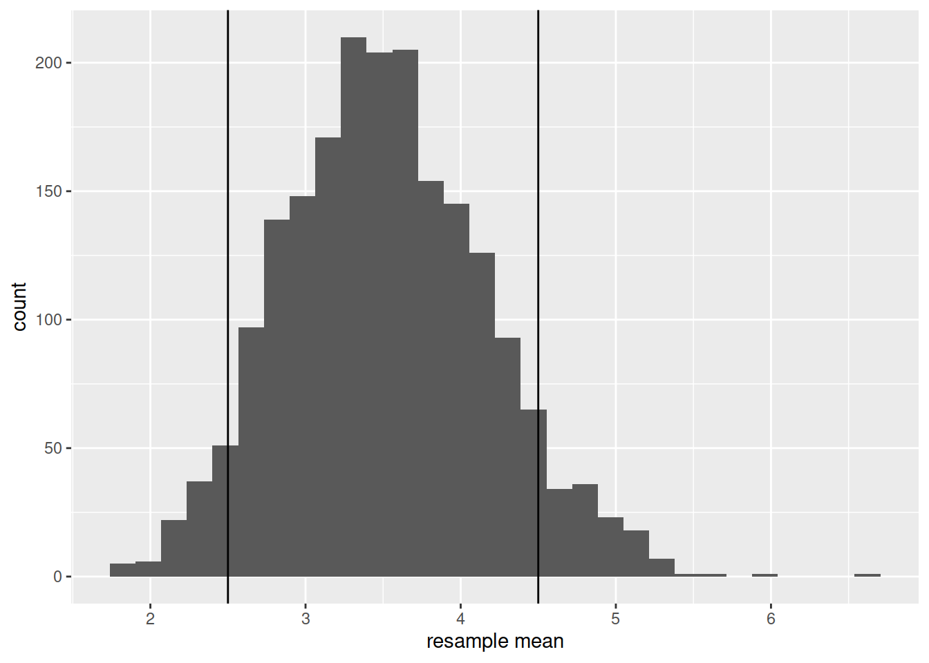
This set of resample means is the bootstrap distribution.
We can plot them:

bootstrap_dist <- 
  rep_sample_n(nfl_sample, n = 50, samples = 2000, replace = TRUE) %>%
  group_by(sample) %>%
  summarise(avg_salary = mean(YearlySalary))

ggplot(bootstrap_dist, aes(x = avg_salary)) + 
  geom_histogram() + 
  labs(x = "resample mean")

Question

Where do you think that this histogram is centred?

• The mean salary of the population (\(\mu\)).
• The mean salary of the original sample (\(\bar{x}\)).
• Somewhere else.

Solution

The distribution of means of resamples will be centered around the mean of our original sample, which was 3.52.

bootstrap_dist %>%
  summarise(mean_of_means = mean(avg_salary))

## # A tibble: 1 x 1
##   mean_of_means
##           <dbl>
## 1          3.52

Question

Last semester we looked at the standard error (the standard deviation of the sampling distribution). The boostrap distribution is an approximation of the sampling distribution.

TRUE or FALSE: The standard deviation of the bootstrap distribution is an approximation of the standard error of \(\bar{x}\).

Solution

TRUE!

More generally…

Now let’s think more generally about what we did there…

1. We were interested in estimating some unknown parameter of a population.
2. We had a sample of size \(n\) drawn at random from the population.
3. We took lots of resamples (of size \(n\)) from our original sample, and calculated a statistic for each one.
4. We then visualised the distribution of those statistics.

The tool below may help to conceptualise these steps:

• The big blue distribution at the top: The population.
  
• The vertical blue line: The population parameter \(\mu\).
• The yellow sample button: Takes a sample from the population (note you can change the sample \(n\)).
• The green resample button: Samples with replacement from the original sample (the yellow one), and calculates the mean (which is then dropped into the bottom panel).
• The bottom panel: The distribution of resample means - the bootstrap distribution!

Spend 10 minutes changing things such as the sample size. If you have any questions about what is happening, then please ask either now or during the lab.

source: https://web.archive.org/web/20160807193104/http://wise1.cgu.edu/vis/bootstrap/

Confidence Intervals

Point estimates & Ranges of Plausible Values

Take a look again at the bootstrap distribution we constructed (Figure 1, below).

Figure 1: Bootstrap resampling distribution based on 2000 resamples

Question

Roughly, between what two values do most of the resample means lie?

Solution

“Most” is very vague. Just eyeballing, most of the distribution lies between 2.5 and 4.5.

ggplot(bootstrap_dist, aes(x = avg_salary)) + 
  geom_histogram() + 
  labs(x = "resample mean")+
  geom_vline(xintercept = c(2.5, 4.5))

Confidence intervals simply answer more exactly where “most” sample means lie - they give us a range of plausible values for our population parameter.

To construct a confidence interval, we need two things:

1. a confidence level;
   
2. a measure of sampling variability.

We have the latter, in the form of our bootstrap distribution. The confidence level, instead, needs to be set by us. For instance, we might ask between which values the middle 95% (or 90%, or 80%, etc.) of our distribution falls. In other words, the confidence level is the “success rate”: the proportion of all samples whose intervals contain the true parameter.

Interpreting a confidence interval?

If we were to do this whole process over and over again:

• take a random sample of size \(n\);
• sample with replacement from that sample;
• construct a 95% confidence interval.

Then about 95% of the confidence intervals we created would contain the population mean.

So if we did this 100 times, we would expect about five of our 95% confidence intervals to not contain the true population mean.

And if we had been constructing 80% confidence intervals instead, we would expect roughly 80 of them to contain the population mean.

Constructing a confidence interval for the mean

We can construct confidence intervals using the standard error. However, we cannot compute standard errors from just one sample, so we need to estimate the standard error of a statistic using either bootstrap, or the formula approach.

We also use the following rules of thumb:

If the distribution is symettric and bell-shaped…

• 68% of values will lie within 1 standard deviation of the mean.
• 95% of values will lie within 1.96 standard deviations of the mean.
• 99.7% of values will lie within 3 standard deviations of the mean.

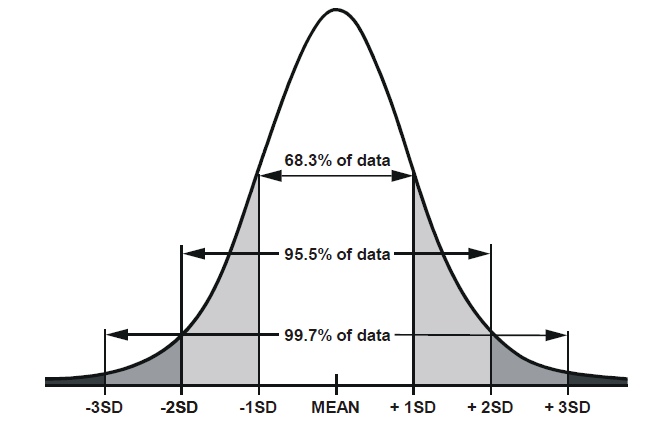
We have our sample mean, and we can calculate the standard deviation of our bootstrap distribution (to approximate the standard error of the sample mean). We therefore have all the information we need to calculate, for instance, a 95% confidence interval - it is \(1.96 \times \text{standard error}\) above and below our mean.

Formally, we can write this 95% interval as:

\(\text{Statistic} \pm 1.96 \times SE\)

Bootstrap SE

The bootstrap standard error is just the standard deviation of the bootstrap distribution which we generated:

sd(bootstrap_dist$avg_salary)

## [1] 0.6511474

So the 95% confidence interval would be the mean of our original sample, plus or minus 1.96 times the bootstrap SE.

mean(nfl_sample$YearlySalary) - 1.96*sd(bootstrap_dist$avg_salary)

## [1] 2.241011

mean(nfl_sample$YearlySalary) + 1.96*sd(bootstrap_dist$avg_salary)

## [1] 4.793509

Does this interval contain the true population parameter? The answer is yes, 95 out of 100 times it will.

Formula approach

Recall the formula for the standard error: \(\text{SE} = \frac{\sigma}{\sqrt{n}}\), where \(\sigma\) is the standard deviation of the population, or our estimate of it (i.e., our sample standard deviation \(\hat \sigma\) or \(s\)), and \(n\) is our sample size.

This will therefore be our estimate of the standard error:

sd(nfl_sample$YearlySalary) / sqrt(50)

## [1] 0.652454

And this will be our 95% confidence interval:

mean(nfl_sample$YearlySalary) - 1.96*(sd(nfl_sample$YearlySalary) / sqrt(50))

## [1] 2.23845

mean(nfl_sample$YearlySalary) + 1.96*(sd(nfl_sample$YearlySalary) / sqrt(50))

## [1] 4.79607

Glossary

• Population. The entire collection of units of interest.

• Sample. A subset of the entire population.

• Parameter. A fixed but typically unknown quantity describing the population.

• Statistic. A quantity computed on a sample.

• Sampling distribution. The distribution of the values that a statistic takes on different samples of the same size and from the same population.

• Standard error. The standard error of a statistic is the standard deviation of the sampling distribution of the statistic.

• Resample. To sample again from your original sample

• Bootstrapping. Repeated random sampling with replacement

• Bootstrap distribution. The distribution of statistics calculated on random resamples. Approximates the sampling distribution of the sample statistic.

• Confidence interval (CI). A range of plausible values around an estimate (e.g., a sample statistic), taking into account uncertainty in the statistic (e.g., sampling variability)

• Confidence level. The percentage of confidence intervals which will contain the true population parameter in the long run (i.e., if you sampled the population and constructed confidence intervals many times over). The proportion of all samples whose intervals contain the true parameter.

Exercises

Remember you will need to “source” the rep_sample_n() function into your environment. Paste this code and make sure it appears in the top-right pane of RStudio.

source('https://uoepsy.github.io/files/rep_sample_n.R')

Hollywood Movies

The following code chunk reads in a sample of the Hollywood movies data we saw last week.

hollywood_sample <- read_csv("https://uoepsy.github.io/data/hollywoodsample1.csv")

Question 1

This week, we’re interested in the average Rotten Tomatoes rating for all Hollywood movies between 2007 and 2013.
What is our best estimate of this with the data we just read in?

Solution

\(\bar{x}\), the mean Rotten Tomatoes rating for our sample.

hollywood_sample %>% 
  summarise(avg_rating = mean(RottenTomatoes))

## # A tibble: 1 x 1
##   avg_rating
##        <dbl>
## 1       49.2

Question 2

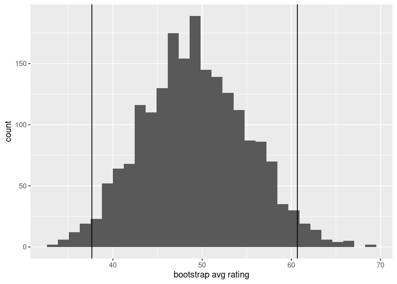
Generate 2000 bootstrap resamples to create the bootstrap distribution. Store it as an object in R with the name hollywood_bs.

Solution

hollywood_bs <- 
  rep_sample_n(hollywood_sample, n = 25, samples = 2000, replace = TRUE) %>%
  group_by(sample) %>%
  summarise(avg_rating = mean(RottenTomatoes))

Question 3

Estimate the standard error of the sample statistic from your bootstrap distribution.

Solution

hollywood_bs %>%
  summarise(estimated_SE = sd(avg_rating))

## # A tibble: 1 x 1
##   estimated_SE
##          <dbl>
## 1         5.88

or

sd(hollywood_bs$avg_rating)

## [1] 5.875942

Question 4

Compute the 95% confidence intervals around our estimate of the average Rotten Tomatoes rating, and plot the bootstrap distribution and the confidence interval.

Hint: geom_vline().

Solution

hwood_ci_lower <- mean(hollywood_sample$RottenTomatoes) - 1.96 * sd(hollywood_bs$avg_rating)
hwood_ci_upper <- mean(hollywood_sample$RottenTomatoes) + 1.96 * sd(hollywood_bs$avg_rating)

ggplot(hollywood_bs, aes(x=avg_rating)) +
  geom_histogram() +
  geom_vline(xintercept = c(hwood_ci_lower, hwood_ci_upper)) +
  labs(x = "bootstrap avg rating")

Question 5

Here is a new sample, but this time it contains 50 movies. Do the same (estimate the mean and construct a confidence interval). How does the confidence interval differ from the one created for a sample of 25?

hollywood_sample2 <- read_csv("https://uoepsy.github.io/data/hollywoodsample2.csv")

Solution

hollywood_sample2 <- read_csv("https://uoepsy.github.io/data/hollywoodsample2.csv")

hollywood_bs <- 
  rep_sample_n(hollywood_sample2, n = 50, samples = 2000, replace = TRUE) %>%
  group_by(sample) %>%
  summarise(avg_rating = mean(RottenTomatoes))

mean(hollywood_sample2$RottenTomatoes) - 1.96 * sd(hollywood_bs$avg_rating)

## [1] 39.88288

mean(hollywood_sample2$RottenTomatoes) + 1.96 * sd(hollywood_bs$avg_rating)

## [1] 54.19712

Question 6

Using the formula approach for the standard error, construct 95% and 99% confidence intervals around the mean Rotten Tomatoes rating based on the sample of 50 movies.

Given that for the 99% confidence interval we will have greater confidence that it will contain the true population parameter than the 95% confidence interval, do we expect the range to be bigger or smaller?

Solution

We are more confident in wider ranges, so the 99% CI will be wider.

Example:

• imagine you are trying to guess my age.
• how confident are you that I am between 25 and 35 years old?
• how confident are you that I am between 10 and 50 years old?
• how confident are you that I am between 29 and 31 years old?
• how confident are you that I am between 0 and 1000 years old?

mean(hollywood_sample2$RottenTomatoes) - 1.96 * (sd(hollywood_sample2$RottenTomatoes)/sqrt(50))

## [1] 39.80105

mean(hollywood_sample2$RottenTomatoes) + 1.96 * (sd(hollywood_sample2$RottenTomatoes)/sqrt(50))

## [1] 54.27895

mean(hollywood_sample2$RottenTomatoes) - 3 * (sd(hollywood_sample2$RottenTomatoes)/sqrt(50))

## [1] 35.95997

mean(hollywood_sample2$RottenTomatoes) + 3 * (sd(hollywood_sample2$RottenTomatoes)/sqrt(50))

## [1] 58.12003

NFL Players

Question 7

Scroll back up - what was the population mean yearly salary for all NFL players at the beginning of 2015?

Solution

nfl_pop <- read_csv("https://uoepsy.github.io/data/nflpop.csv")
mean(nfl_pop$YearlySalary)

## [1] 3.033404

3.03 (million dollars!!)

Question 8

A researcher lives in Boston. They want to estimate salaries of NFL players, and in 2015 they go around and ask 50 players about their yearly salaries.
The code below reads in the sample they collected.

nfl_boston <- read_csv("https://uoepsy.github.io/data/nflboston.csv")

Compute the sample mean, and calculate 95% confidence intervals via bootstrap standard error

Solution

nfl_bs <- rep_sample_n(nfl_boston, n = 50, samples = 2000, replace = TRUE) %>%
  group_by(sample) %>%
  summarise(avg_salary = mean(YearlySalary))

mean(nfl_boston$YearlySalary) - 1.96 * sd(nfl_bs$avg_salary)

## [1] 1.412244

mean(nfl_boston$YearlySalary) + 1.96 * sd(nfl_bs$avg_salary)

## [1] 2.862436

Question 9

This confidence does not include the population mean of 3.03. Why not?

ggplot(nfl_bs, aes(x=avg_salary)) +
  geom_histogram() +
  labs(x = "bootstrap avg salary (millions of $)\nbased on bootstrapped Boston sample") +
  geom_vline(xintercept = mean(nfl_pop$YearlySalary))+
  geom_text(x=3.05, y=150,label="True population mean",hjust=0)+
  geom_vline(xintercept = c(mean(nfl_boston$YearlySalary) - 1.96 * sd(nfl_bs$avg_salary), mean(nfl_boston$YearlySalary) + 1.96 * sd(nfl_bs$avg_salary)), col="tomato1")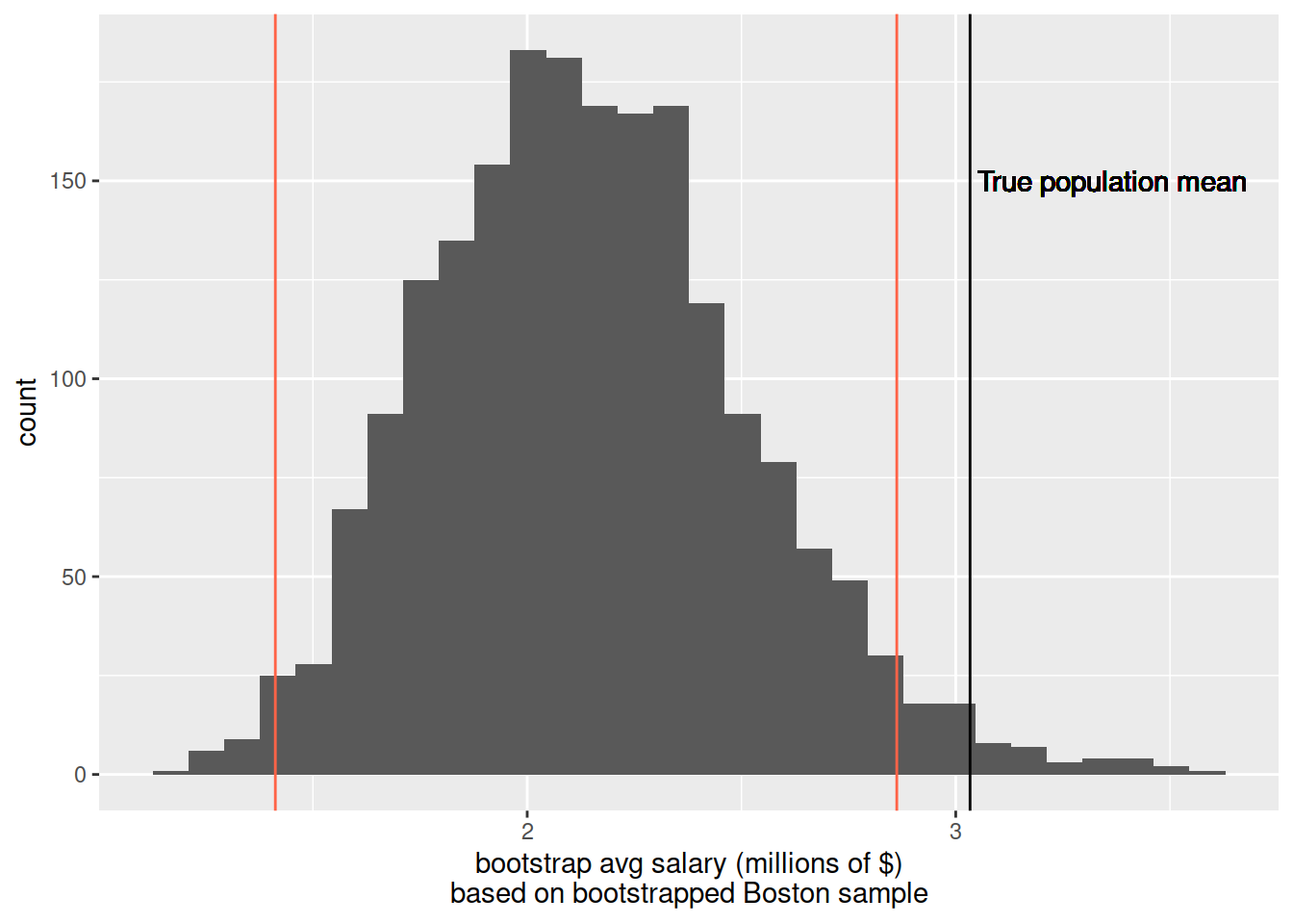

Hint: Look at your data, and think about what you know about how it was collected - why might this not be a good sample?

Solution

The researcher, living in Boston, seems to have sampled a lot of players from the New England Patriots (a local team).

The key thing here is that the statistical inference we are making (that the sample mean is an estimate of the population mean) assumes that the sample is an unbiased representation. In this case it is not a truly random sample!