What does it mean to “compile” a document?
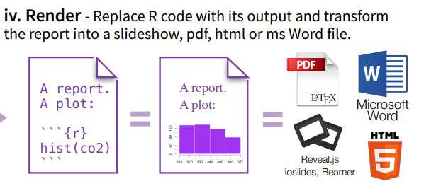
Figure 1: Rendering (from https://www.rstudio.com/wp-content/uploads/2015/02/rmarkdown-cheatsheet.pdf)
Often, when talking about “compiling” RMarkdown documents, you will find different words used for this process, such as “compiling”, “rendering”, and “knitting”.
The basic idea is that we are turning the .rmd file we are editing in RStudio into something much more reader-friendly, such as a .pdf, or an .html, or even a word file .docx.

If you open up the .rmd file from Lesson 1, and click the “knit” icon at the top of the document, you see lots of stuff happening below, and then a nicely formatted document will pop-up. (Note: If you have not already saved your RMarkdown document (hopefully you have!), then when you click “knit”, it will prompt you to save it first.)
You may find that the document pops up in a separate window, or in the “viewer” pane in the bottom right of RStudio.
You can control this behaviour by looking in the top menu of RStudio for “Tools” > “Global Options” > “RMarkdown” > “Show output preview in:”.
Compiled Files
The compiled file will be in the same folder as where you have saved your .rmd file. If you are using an “Project”, or have set your working directory using setwd() (see r-bootcamp Lesson 2) then you can fine these easily in the Files tab of RStudio. You can also find these in your file-browser that you use to find all your other files on your computer.
You should now have TWO files on your computer with the same name but one is an .Rmd and one is a .html. You could email the .html file to someone and they could open it in their web browser. The .Rmd file can only be opened and understood by someone who has access to R.
Compiling and Sessions/Environments
When an RMarkdown document gets compiled, it does so as a self-contained process. This ensures reproducibility!
It doesn’t matter what you can see in your Environment, nor what packages you have loaded.
What matters is what is in the RMarkdown document.
When you click “knit”, the lines of code in your RMarkdown document will be evaluated one-by-one, and the document must contain everything required to evaluate each line.
For example:
- if you have not got a line in your document that loads the tidyverse packages, then you will not be able to use functions like
group_by(),filter,%>%etc in the document, because it won’t know where to find them.
- if you have not got the line that loads the tidyverse packages before you use functions like
group_by(),filter,%>%etc, then it won’t know where to find them.
Where is the RMarkdown looking for objects/functions, if not your environment? It’s looking in its own environment!
The “setup” chunk
Because compiling an RMarkdown document requires everything necessary for all the code to run without errors to be included in the document and in the correct order, there is an optimum way to structure your document.
Immediately after the metadata (title, author etc), we specify the “setup” chunk (see below). In the setup chunk, we typically load all the packages we rely on in the rest of the document, so that they get loaded first.1 It is also typical to use this chunk to read in your data.
You can see an example below.
---
title: "this is my title"
author: "I am the author"
date: "13/08/2021"
output: html_document
---
```{r setup, include = FALSE}
library(tidyverse)
library(palmerpenguins)
somedata <- read_csv(“https://edin.ac/2wJgYwL”)
```
Instead of
```{r}
```{r setup, include = FALSE}
setup is simply the name of our code-chunk. We can call it anything we want, for instance:```{r peppapig}
The second bit, the include = FALSE is what is known as a “chunk-option”, and we will get to these later on. What this does is basically mean that neither this chunk of code nor its output will be visible in the compiled document.
Don’t use
install.packages()here - or it will re-install the package every time you compile. Just useinstall.packages()in the console.↩︎