Prelude
Remember in the lesson on compiling, we saw that it is typical to have a “setup” code-chunk at the start of your document, in which you load all the packages you need, and read in the data etc.
A normal code-chunk looks like:
 ```{r}

 ```
And we had a special chunk which looked like:
 ```{r setup, include = FALSE}

 ```
Chunk name
The first thing to note is that we can give our code-chunks a name.
This is usually the first thing inside the {} after the letter “r”:
 ```{r mychunkname}

 ```
This will come in handy later on when we want to reference the output from certain code-chunks. One immediate benefit is that you can easily navigate through your document to get to the code-chunk you want, by using the menu in the bottom-left of the editor in RStudio:
[insert video of chunk scrolling]
Chunk options
Along with providing a name for each code-chunk, we can specify how we want it to compile in our finished document. For instance, do we want the code to be shown in the document? Do we want the output to be shown? Do we even want the code to be evaluated, or do we want R to skip over it? These things are all controlled via “chunk options”.
Setting code chunk options inside {}
The most straightforward way to set the options for a given code-chunk is to include it inside the {} bits of the code-chunk.
In the code-chunk below (named “mychunkname”), we have set include = FALSE inside the squiggly-brackets {}. This means that for this code-chunk, the include option will be set as FALSE (we’ll learn what that actually does in just a minute!).
 ```{r mychunkname, include = FALSE}
 plot(mtcars)
 ```
echo = ?
the “echo” option sets whether or not the code is printed to the compiled document. It doesn’t change whether the code gets evaluated, and it doesn’t change whether the output (e.g. plots, tables, printed objects) get shown, it just hides/shows the code from the finished document. You can see an example below.
echo = TRUE
Writing this:
 ```{r mychunkname, echo = TRUE}
 pass_scores <- read.csv(“https://edin.ac/2wJgYwL”)
 barplot(table(pass_scores$school))
 ```
Will compile to this:

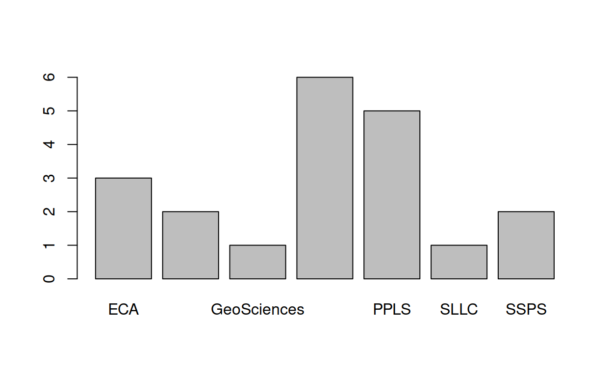
echo = FALSE
Writing this:
 ```{r mychunkname, echo = FALSE}
 pass_scores <- read.csv(“https://edin.ac/2wJgYwL”)
 barplot(table(pass_scores$school))
 ```
Will compile to this:

eval = ?
The “eval” option sets whether or not a code-chunk will be evaluated. For instance, if you set one chunk to not be evaluated, then the resulting computations inside that code-chunk will not happen, and when compiling the document, subsequent chunks which depend on that chunk will be altered. You can see an example of this below.
eval = TRUE
Writing this:
 ```{r mychunkname, eval = TRUE}
 pass_scores <- read.csv(“https://edin.ac/2wJgYwL”)
 ```
 ```{r mychunk2}
 barplot(table(pass_scores$school))
 ```
Will compile to this:
pass_scores <- read.csv("https://edin.ac/2wJgYwL")

eval = FALSE
Writing this:
 ```{r mychunkname, eval = FALSE}
 pass_scores <- read.csv(“https://edin.ac/2wJgYwL”)
 ```
 ```{r mychunk2}
 barplot(table(pass_scores$school))
 ```
Will compile to this:
pass_scores <- read.csv("https://edin.ac/2wJgYwL")
include = ?
The include option is a bit of a funny one. It will not change whether the code gets evaluated, but it will mean all the output (and the code) will be hidden from the compiled document. This is a useful way of making sure that some necessary code does get run when compiling the document, but everything (code + output) gets hidden.
include = TRUE
Writing this:
 ```{r mychunkname, include = TRUE}
 pass_scores <- read.csv(“https://edin.ac/2wJgYwL”)
 mytable <- table(pass_scores$school)
 mytable
 ```
 ```{r mychunk2}
 barplot(mytable)
 ```
Will compile to this:
        ECA   Economics GeoSciences         LAW        PPLS
          3           2           1           6           5
       SLLC        SSPS
1 2 barplot(mytable)

include = FALSE
Writing this:
 ```{r mychunkname, include = FALSE}
 pass_scores <- read.csv(“https://edin.ac/2wJgYwL”)
 mytable <- table(pass_scores$school)
 mytable
 ```
 ```{r mychunk2}
 barplot(mytable)
 ```
Will compile to this:
barplot(mytable)
warning = ? and message = ?
These are perhaps the most intuitive of the chunk options to remember. Some lines of code will return a message, some will return a warning. These chunk options simply control whether or not they get shown in the final compiled document.
message = TRUE
Writing this:
 ```{r mychunkname, message = TRUE}
 library(tidyverse)
 ```
Will compile to this:
message = FALSE
Writing this:
 ```{r mychunkname, message = FALSE}
 library(tidyverse)
 ```
Will compile to this:
warning = TRUE
Writing this:
 ```{r mychunkname, warning = TRUE}
 x <- c(“2”, -3, “end”, 0, 4, 0.2)
 as.numeric(x)
 ```
Will compile to this:
x <- c("2", -3, "end", 0, 4, 0.2)
as.numeric(x)
Warning: NAs introduced by coercion[1] 2.0 -3.0 NA 0.0 4.0 0.2warning = FALSE
Writing this:
 ```{r mychunkname, warning = FALSE}
 x <- c(“2”, -3, “end”, 0, 4, 0.2)
 as.numeric(x)
 ```
Will compile to this:
x <- c("2", -3, "end", 0, 4, 0.2)
as.numeric(x)
[1] 2.0 -3.0 NA 0.0 4.0 0.2Global options
As well as being able to set the options for specific code-chunks, we can set them globally for all the code-chunks in our document.
We can do this inside a code-chunk (seems weird, I know!), code like this in our first chunk (the “setup” chunk):
 ```{r setup, include = FALSE}
 library(knitr) opts_chunk$set(echo = FALSE, message = FALSE)
 ```
This will mean that for all subsequent code-chunks, the code will not get printed in the final document, and no messages will get printed either (this is unless we specifically set echo = TRUE for a code-chunk later on, which will override the global option).