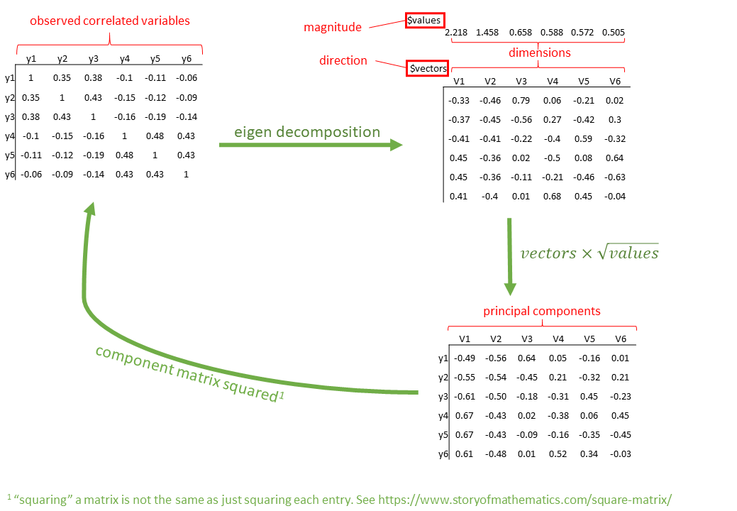
Using principal() from the {{psych}} package, with 8 observed variables, we are working in 8 dimensions. These observed variables are all correlated, and PCA re-expresses the information onto un-correlated (i.e. perpendicular) dimensions.
This is achieved using “eigen decomposition” which is a fairly complex calculation performed on the correlation matrix.
With \(p\) variables, we can get out \(p\) orthogonal dimensions, which here we call “principal components”. In the principal() function, we can set nfactors = 8 to extract 8 dimensions.1
Because the process of eigen decomposition is essentially just a re-expression of our correlation matrix, we if we take our 8 principal components all together, we are explaining all of the variance in the original data. In other words, the total variance of the principal components (the sum of their variances) is equal to the total variance in the original data (the sum of the variances of the variables). This makes sense - we have simply gone from having 8 correlated variables to having 8 orthogonal (unrelated) components - we haven’t lost any variance.
The key benefit of PCA is that our orthogonal components have sequential variance maximisation - i.e., the first captures the most variance, then the second captures the second most, and so on.. So if we just want to reduce down to 1 dimension, then we just keep the first component. If we want to keep some pre-specified amount (e.g., 80%) of variability, then accessing Vaccounted will give us information on the amount of variance captured by each component:
SS loadings: The sum of the squared loadings (these are also the “eigenvalues”). These represent the amount of variance explained by each component, out of the total variance (which is 8, because we have 8 variables (the variables are all standardised, meaning they each have a variance of 1. \(8 \times 1 = 8\) so we can think of the total variance as 8!)
Proportion Var: The proportion the overall variance the component accounts for out of all the variables.
Cumulative Var: The cumulative sum of Proportion Var.
Proportion Explained: relative amount of variance explained (\(\frac{\text{Proportion Var}}{\text{sum(Proportion Var)}}\).
Cumulative Proportion: cumulative sum of Proportion Explained.
There are lots of methods to help us decide how many components we should keep.
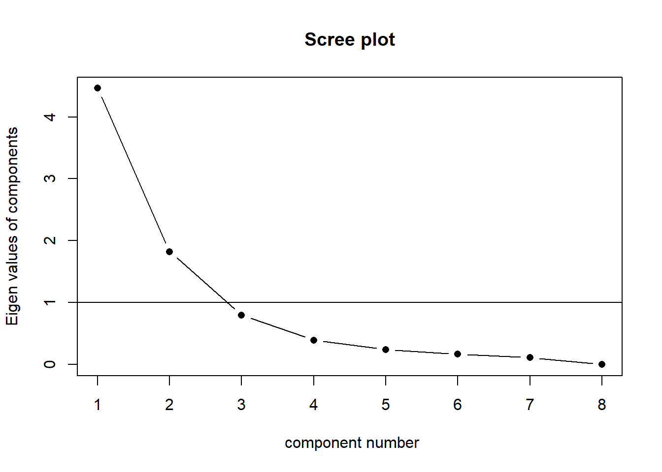
Scree plot
Scree plots show the eigenvalues for each component (each new dimension). A typical scree plot features higher variances for the initial components and quickly drops to small variances where the curve is almost flat. The flat part of the curve represents the noise components, which are not able to capture the main sources of variability in the system.
According to the scree plot criterion, we should keep as many principal components up to where the “kink” (or “elbow”) in the plot occurs. So in the above plot, the kink occurs at 3 by my reckoning (yours might be different!), so I would keep 2.
NOTE: Scree plots are subjective and may have multiple or no obvious kinks/elbows, making them hard to interpret
scree(physfunc[,1:8], pc =TRUE, factors =FALSE)
The horizontal line is an additional suggestion that we should keep all components for which the eigenvalue is >1. This is known as “Kaiser’s Criterion”
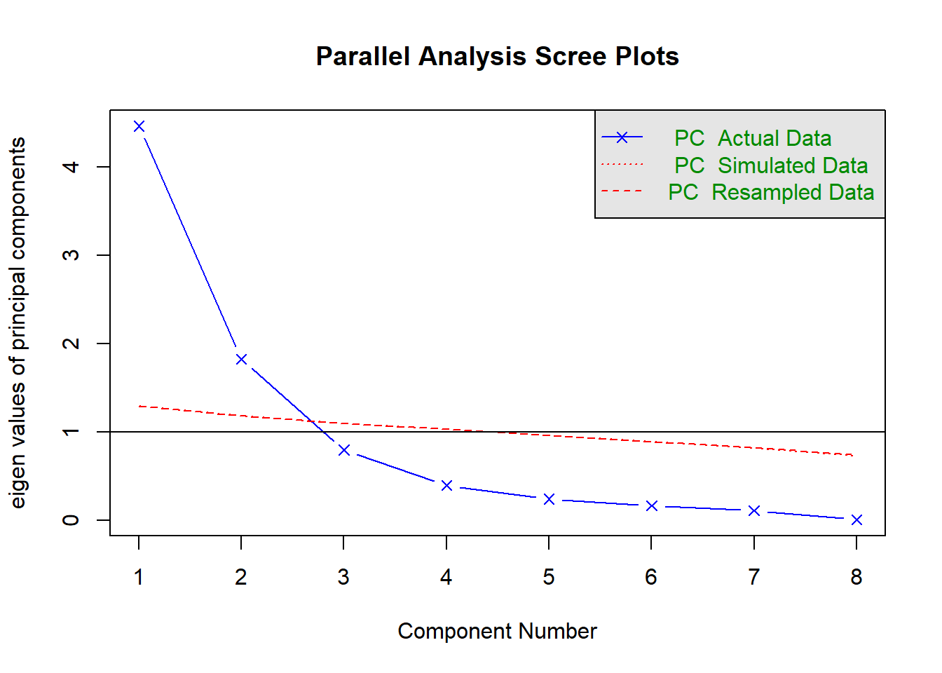
Parallel analysis
Parallel analysis involves simulating lots of datasets of the same dimension but in which the variables are uncorrelated. For each of these simulations, a PCA is conducted on its correlation matrix, and the eigenvalues are extracted. We can then compare our eigenvalues from the PCA on our actual data to the average eigenvalues across these simulations. In theory, for uncorrelated variables, no components should explain more variance than any others, and eigenvalues should be equal to 1. In reality, variables are rarely truly uncorrelated, and so there will be slight variation in the magnitude of eigenvalues simply due to chance. The parallel analysis method suggests keeping those components for which the eigenvalues are greater than those from the simulations.
It can be conducted in R using the fa.parallel() function.
When conducting an EFA (we’ll see this later on in these readings) as opposed to a PCA, you can set fa = "both" to do this for both factor extraction and principal components.
fa.parallel(physfunc[,1:8], fa ="pc", n.iter =500)
Parallel analysis suggests that the number of factors = NA and the number of components = 2
NOTE: Parallel analysis will sometimes tend to over-extract (suggest too many components)
MAP
The Minimum Average Partial (MAP) test computes the partial correlation matrix (adjusting for and removing a component from the correlation matrix), sequentially partialling out each component. At each step, the partial correlations are squared and their average is computed.
At first, the components which are removed will be those that are most representative of the shared variance between 2+ variables, meaning that the “average squared partial correlation” will decrease. At some point in the process, the components being removed will begin represent variance that is specific to individual variables, meaning that the average squared partial correlation will increase.
The MAP method is to keep the number of components for which the average squared partial correlation is at the minimum.
We can conduct MAP in R using the VSS() function.
library(psych)VSS(physfunc[,1:8], rotate ="none", plot =FALSE, fm ="pc")
Very Simple Structure
Call: vss(x = x, n = n, rotate = rotate, diagonal = diagonal, fm = fm,
    n.obs = n.obs, plot = plot, title = title, use = use, cor = cor)
VSS complexity 1 achieves a maximimum of 0.96  with  2  factors
VSS complexity 2 achieves a maximimum of 0.99  with  3  factors

The Velicer MAP achieves a minimum of 0.14  with  1  factors
BIC achieves a minimum of Inf with factors
Sample Size adjusted BIC achieves a minimum of  Inf  with    factors

Statistics by number of factors
  vss1 vss2  map dof chisq prob sqresid  fit RMSEA BIC SABIC complex eChisq
1 0.83 0.00 0.14   0    NA   NA 4.2e+00 0.83    NA  NA    NA      NA     NA
2 0.96 0.96 0.15   0    NA   NA 8.9e-01 0.96    NA  NA    NA      NA     NA
3 0.72 0.99 0.19   0    NA   NA 2.5e-01 0.99    NA  NA    NA      NA     NA
4 0.59 0.91 0.28   0    NA   NA 9.8e-02 1.00    NA  NA    NA      NA     NA
5 0.67 0.89 0.43   0    NA   NA 3.9e-02 1.00    NA  NA    NA      NA     NA
6 0.67 0.88 0.83   0    NA   NA 1.2e-02 1.00    NA  NA    NA      NA     NA
7 0.54 0.78 1.00   0    NA   NA 2.8e-05 1.00    NA  NA    NA      NA     NA
8 0.54 0.78   NA   0    NA   NA 1.3e-28 1.00    NA  NA    NA      NA     NA
  SRMR eCRMS eBIC
1   NA    NA   NA
2   NA    NA   NA
3   NA    NA   NA
4   NA    NA   NA
5   NA    NA   NA
6   NA    NA   NA
7   NA    NA   NA
8   NA    NA   NA
There is a lot of other information in this output too! For now just focus on the map column, and the part of the output that says “The Velicer MAP achieves a minimum of 0.14 with 1 factors”.
This statement tells us that the minimum average squared partial correlation is achieved for 1 factor, which means that MAP suggests we keep only one factor. (The map column shows us the average squared partial correlation for each number of factors, and the MAP test will find the lowest value in that column and recommend to us the corresponding number of factors.)
NOTE: The MAP method will sometimes tend to under-extract (suggest too few components)
Loadings
Supposing that we decide (based on the scree plot, parallel analysis and MAP) to retain two components, capturing 79% of the total variance, the “loadings” tell us how each component is related back to the original variables.
So in the case below, we can see that the first component is positively related to most of the variables apart from endurance (it’s small and negative) and respiratory (it’s not even shown because it’s so small). The second component is related positively to both of these variables, and not clearly related to the others.
Note: As soon as we start to examine the loadings and try to give some sort of meaning to the components, we are going away from a pure form of PCA, and using it more like exploratory factor analysis, which we will see more of below and in the next chapter
Scores
When it comes to using the principal components in some subsequent analysis, we need to access the “scores”.
Scores in PCA represent the relative standing of every observation in our dataset on each component.
These are essentially weighted combinations of an individual’s values on the original variables. \[
\text{score}_{\text{component j}} = w_{1j}y_1 + w_{2j}y_2 + w_{3j}y_3 +\, ... \, + w_{pj}y_p
\] Where \(w\) are the weights, \(y\) the original variable scores.
Optional: How are weights calculated?
The weights are calculated from the eigenvectors as \[
w_{ij} = \frac{a_{ij}}{\sqrt{\lambda_j}}
\] where \(w_{ij}\) is the weight for a given variable \(i\) on component \(j\) , \(a_{ij}\) is the value from the eigenvector for item \(i\) on component \(j\) and \(\lambda_{j}\) is the eigenvalue for that component.
The correlations between the scores and the measured variables are what we saw in the “loadings”!