2: Dimension Reduction
This reading:
- build the intuition for thinking about “dimensions” of data
- introduce some key goals and methods that researchers use, and how these differ in relation to finding and using dimensions of data
The dimensionality of data
Take a moment to think about the various things that you are often interested in when discussing psychology. This might be anything from personality traits, to language proficiency, social identity, anxiety etc. How we measure such constructs is a very important consideration for research. The things we’re interested in are very rarely the things we are directly measuring.
Consider how we might assess levels of anxiety or depression. Can we ever directly measure anxiety?1 More often than not, we measure these things using a set of different measures which ‘look at’ the underlying construct from a different angle. In psychology, this is often questionnaire based methods, with a set of questions each of which might ask about “anxiety” from a slightly different angle. Twenty questions all measuring different aspects of anxiety are (we hope) going to correlate with one another if they are capturing some commonality (the construct of “anxiety”).
But this introduces a problem for us, which is how to deal with 20 variables that represent (in broad terms) the same single thing. How can we talk about “changes in anxiety”, and not just “changes on anxiety Q1” and “changes on anxiety Q2” and so on? In addition, not all of these constructs will necessarily exist as one distinct thing - we often talk about “narcissm”, but this could arguably be comprised of 3 slightly distinct constructs of “grandiosity”, “vulnerability” and “antagonism”.
What we are touching upon here gets referred to as dimensionality of a measurement tool, and the questions we are going to look at are all about how we can go from the big set of observed variables to the key things that are the things we are actually interested in.
What is a “dimension”?
Broadly speaking, when we use the term “dimension” here, we are more or less referring to something like the number of rows and columns in a dataset. If I measure \(n\) people on 10 questions about anxiety, then my resulting dataset will have $n $10 dimensions.
But in many cases this contrasts with our research questions, which are concerned with a construct (e.g., the idea of “anxiety”) that we consider to be a single dimension (e.g., people are high on anxiety or low on anxiety) rather than 10.
When might we want to reduce dimensionality?
There are many reasons we might want to “reduce the dimensionality” of data:
- Pragmatic
- I have multicollinearity issues/too many variables, how can I defensibly combine my variables?
- Test construction
- How should I group my questionnaire items into subsets?
- Which items are the best measures of my construct(s)?
- Theory testing
- What are the number and nature of dimensions that best describe a theoretical construct?
The core idea
Let’s suppose we are interested in capturing how tired people are, and we had data on three different related variables:
- Subjective Mental Fatigue
- Subjective Physical Fatigue
- Subjective Sleepiness
We might visualise these in the 3-dimensional space of the measured variables in Figure 1.
Although we have measured 3 variables, when faced with trying to characterise the shape of the 3-dimensional cloud of datapoints, we’re more inclined to think about its length, width and depth. You can imagine trying to characterise this shape as the ellipse in Figure 2. It looks a little like a bar of soap or something! It’s longer in one direction (green line), wide in another direction (red line), and not very deep (blue line). We can think of these as some new “dimensions” that we could also use to characterise the shape of data.
the correlation matrix
The example here has 3 variables, which means 3-dimensions, and this is why we can actually visualise it. But we could also think of this shape as being described by all the correlations between each pair of variables. Each of these correlations is characterising the plot of each pair of variables, and these are just like viewing the 3-d plot above but looking at it from straight on at each side.2 So in cases where we have lots and lots of variables, we might not be able to visualise the n-dimensional shape itself, but we can look at it from all different angles through the correlation matrix!
cor(mydata) M P S
M 1.0000000 0.5981510 0.7488493
P 0.5981510 1.0000000 0.7669584
S 0.7488493 0.7669584 1.0000000pairs(mydata)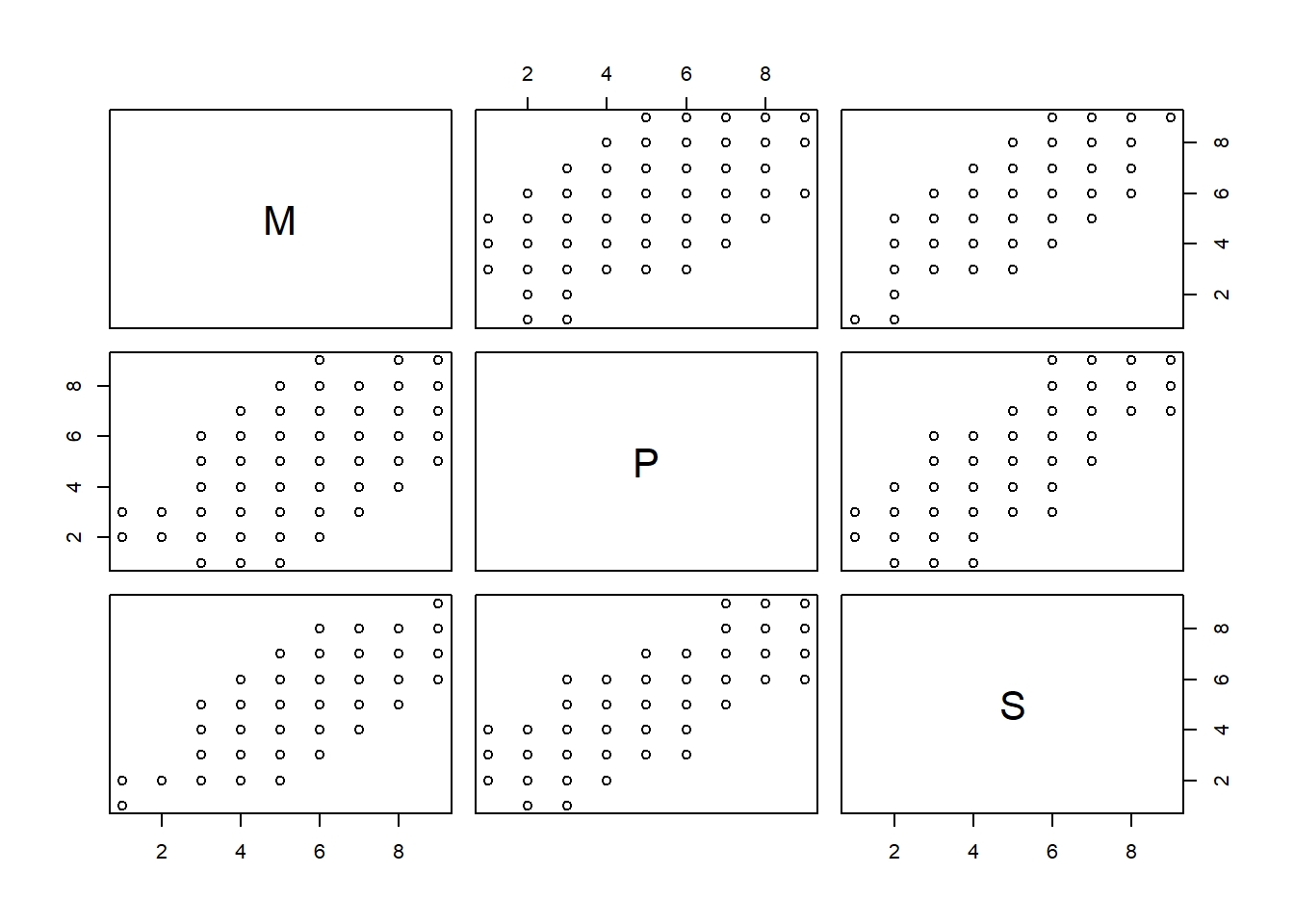
Think a little about what these new dimensions (the coloured axes in Figure 2) represent - they capture “the ways in which observations vary” across the set of observed variables.
The long dimension captures that all three variables tend to co-vary (there are lots of people who are high on all of them, and lots who are low on all of them - there aren’t many who might rate one question an 8 and the other two questions a 2).
One way to see this is to just follow the green line to each end of the ellipse and figure out roughly what the scores would be at that point. At one end of the green line we have people scoring 2 on all 3 variables, and at the other end we have them scoring 8 on all 3.
The next longest dimension of the ellipse (the red line) shows another form of variability - there are people with similar sleepiness scores but some people are high on physical fatigue and low on mental fatigue, and others are low on physical fatigue but high on mental fatigue (i.e., at one end of the red line we have scores of M=8, P=2, S=4, and at the other end we have M=2, P=8, S=4).
Finally the blue dimension of the ellipse is the shortest, capturing the least variability. This dimension seems to differentiate between people who are more sleepy but less fatigued, and those who are less sleepy but more fatigued. It makes sense that there isn’t much variability here - we would expect people who are sleepy to be fatigued and vice versa!
Often it helps to take this to the extremes, so think about what these would look like if we no correlations or perfect correlations between the three variables. If the variables are uncorrelated, then we have a sort of spherical cloud of data, and for any set of three dimensions we try to use to express this shape there is not going to be any one dimension that is longer than the other (Figure 3). By contrast, if we have perfect correlations between the variables, then we actually don’t even need 3 dimensions to express it - we only really need one dimension - we just have a line upon which all observations fall (Figure 4).
The core idea of dimension reduction is that we can re-express our dataset in a new set of dimensions, where we can decide to keep fewer of them and still capture a lot of the shape of the data.
For an analogy, imagine being given a ruler and being asked to give two numbers to provide a measurement of your smartphone. What do you pick? I would take a bet that you will measure its length and then its width. You’re likely to ignore the depth because it is much smaller than the other two dimensions. This is pretty much the concept of dimension reduction.
The idea here is that we can — without losing too much — preserve the general shape of our data using fewer dimensions. Ignoring the depth of our cloud of datapoints, we could reduce from 3 variables down to 2 dimensions by considering where our data falls when projected onto the 2-dimensional surface shown in Figure 5. Or we could reduce down to 1 dimension and consider where the data falls on the single axis shown in Figure 6.
The conceptual idea of these new ‘dimensions’ that we’re working with here is pretty abstract, and it only gets weirder to think about when we have more than 3 variables and we can no longer easily visualise it.
The key thing we are doing here is:
- Identify the dimensions that capture (co)variability across a set of measured variables
- Retain a subset of those dimensions
Depending upon what the goal of our research is, the key questions are going to be:
- how do we find the dimensions?
- how many dimensions should we retain?
- how does each dimension relate back to the original measured variables?
The key methods
Naive ‘Scale Scores’
Goal: Pragmatic. I want 1 thing to use in some other setting (e.g., in a further analysis, or in a clinical setting)
- How do we find the dimensions?
- There’s only one
- How many dimensions should we retain?
- There’s only one
- How does each dimension relate back to the original measured variables?
- All variables equally related to dimension
For example, the AQ10 is a ten-question survey which (despite some well-established issues) is used by the NHS for autism screening. Participants essentially respond “agree” or “disagree” to each question, and the result is scored by summing up the number of responses in the expected direction. People must score above a 6 in order to be referred for autism diagnosis on the NHS.
This is a naive scale score, because there is only one dimension (some measure of autism), and all questions are assumed to be equally related to this dimension.
Code demonstration
Typically scale scores are either mean scores or sum scores. These are, for each person, the mean, or the sum, of their scores on each item.
Because we are wanting this for each person, and each person is a row in our dataset, so we want row means, or row sums.
somedata$meanscore <- rowMeans(somedata[,1:6])
somedata$sumscore <- rowSums(somedata[,1:6])
Principal Component Analysis (PCA)
Goal: Pragmatic. I want fewer things for use in a subsequent analysis but don’t want to lose too much variability. I want those things to be uncorrelated.3
- How do we find the dimensions?
- Set of orthogonal (i.e., perpendicular4 therefore uncorrelated) dimensions that sequentially capture most variability.
- Found via some complicated maths that feels a bit like magic! It utilises a method called “eigen decomposition”, the details of which are beyond the scope of this course, but the high level idea is given below.
- How many dimensions should we retain?
- Pragmatic: defined by either the number of dimensions we want, or the proportion of variability we want to retain
- Tools (detailed in the PCA Walkthrough) such as scree plots, parallel analysis and minimum average partial (MAP) can guide us towards how many dimensions capture a “substantial” amount of variability in the data.
- how does each dimension relate back to the original measured variables?
- Examine correlations between dimensions and variables
- Somewhat irrelevant for ‘pure’ PCA, where we are agnostic/don’t care about what the dimensions are.
Exploratory Factor Analysis (EFA)
Goal: Exploratory/Discovery/Measure development. I don’t have a strong theoretical model yet, but I suspect there are underlying constructs that explain why these variables correlate with each other. I want to discover what those constructs might be and how the variables relate to them.
- How do we find the dimensions?
- Estimation
- Models with different numbers of (possibly correlated) latent dimensions are compared
- How many dimensions should we retain?
- The model that “best explains” our observed relationships between variables
- “best explains” = a theoretical question as much as a numerical one!
- How does each dimension relate back to the original measured variables?
- Examine “loadings” between dimensions and variables
Confirmatory Factor Analysis (CFA)
Goal: Theory testing. I have a theoretical model of how these variables relate to these constructs. I want to test how well that model is reflected in these data
- How do we find the dimensions?
- We define them
- How many dimensions should we retain?
- Irrelevant as the dimensions are pre-defined
- How does each dimension relate back to the original measured variables?
- Pre-defined mapping of which variables to which dimensions. Magnitudes and directions are estimated.
Footnotes
Even if we cut open someone’s brain, it’s unclear what we would be looking for in order to ‘measure’ it. It is unclear whether anxiety even exists as a physical thing, or rather if it is simply the overarching concept we apply to a set of behaviours and feelings.↩︎
Rotate the 3-d plot to make it match the 2-d plots below!↩︎
I might want this if, e.g., I have issues with multicollinearity of predictors in a regression model↩︎
like all those that we’ve seen above↩︎