optional extra: eigen decomposition

A correlation matrix is a square matrix (i.e. same number of columns as rows), and it is symmetric on the diagonals. Furthermore, the diagonal values themselves are all 1 (the correlation of a variable with itself is 1).

So we might see a correlation matrix (lets call it \(\mathbf{R}\)) that looks like this:

\[ \begin{equation*} \mathbf{R} = \begin{bmatrix} 1.00, 0.72, 0.63, 0.54, 0.45, 0.36 \\ 0.72, 1.00, 0.56, 0.48, 0.40, 0.32 \\ 0.63, 0.56, 1.00, 0.42, 0.35, 0.28 \\ 0.54, 0.48, 0.42, 1.00, 0.30, 0.24 \\ 0.45, 0.40, 0.35, 0.30, 1.00, 0.20 \\ 0.36, 0.32, 0.28, 0.24, 0.20, 1.00 \\ \end{bmatrix} \end{equation*} \]

One way in which we can create a symmetric square matrix is to take the product of some vector \(\mathbf{f}\) with \(\mathbf{f'}\) (\(\mathbf{f}\) “transposed”). This is just how you might “square” a vector. To multiply two vectors you take each entry of the first and multiply it with each entry of the second.

For instance:
\[ \begin{equation*} \mathbf{f} = \begin{bmatrix} 0.88 \\ 0.83 \\ 0.77 \\ 0.69 \\ 0.60 \\ 0.50 \\ \end{bmatrix} \qquad \mathbf{f} \mathbf{f'} = \begin{bmatrix} 0.88 \\ 0.83 \\ 0.77 \\ 0.69 \\ 0.60 \\ 0.50 \\ \end{bmatrix} \begin{bmatrix} 0.88, 0.83, 0.77, 0.69, 0.60, 0.50 \\ \end{bmatrix} \qquad = \qquad \begin{bmatrix} 0.78, 0.74, 0.68, 0.61, 0.53, 0.44 \\ 0.74, 0.69, 0.64, 0.58, 0.50, 0.42 \\ 0.68, 0.64, 0.59, 0.53, 0.47, 0.39 \\ 0.61, 0.58, 0.53, 0.48, 0.42, 0.35 \\ 0.53, 0.50, 0.47, 0.42, 0.37, 0.30 \\ 0.44, 0.42, 0.39, 0.35, 0.30, 0.25 \\ \end{bmatrix} \end{equation*} \]

Note that I’ve chosen values for \(\mathbf{f}\) that get pretty close to re-creating \(\mathbf{R}\) (clever me!). I can get even closer if I take this and add to it the product of another vector:

\[ \begin{align} \begin{bmatrix} 0.78, 0.74, 0.68, 0.61, 0.53, 0.44 \\ 0.74, 0.69, 0.64, 0.58, 0.50, 0.42 \\ 0.68, 0.64, 0.59, 0.53, 0.47, 0.39 \\ 0.61, 0.58, 0.53, 0.48, 0.42, 0.35 \\ 0.53, 0.50, 0.47, 0.42, 0.37, 0.30 \\ 0.44, 0.42, 0.39, 0.35, 0.30, 0.25 \\ \end{bmatrix} &+ \begin{bmatrix} 0.06 \\ 0.07 \\ 0.09 \\ 0.13 \\ 0.27 \\ -0.85 \\ \end{bmatrix} \begin{bmatrix} 0.06, 0.07, 0.09, 0.13, 0.27, -0.85 \\ \end{bmatrix} \qquad = \qquad \\ \quad \\ \quad \\ \begin{bmatrix} 0.78, 0.74, 0.68, 0.61, 0.53, 0.44 \\ 0.74, 0.69, 0.64, 0.58, 0.50, 0.42 \\ 0.68, 0.64, 0.59, 0.53, 0.47, 0.39 \\ 0.61, 0.58, 0.53, 0.48, 0.42, 0.35 \\ 0.53, 0.50, 0.47, 0.42, 0.37, 0.30 \\ 0.44, 0.42, 0.39, 0.35, 0.30, 0.25 \\ \end{bmatrix} &+ \begin{bmatrix} 0.00, 0.00, 0.00, 0.01, 0.02, 0.05 \\ 0.00, 0.00, 0.01, 0.01, 0.02, 0.06 \\ 0.00, 0.01, 0.01, 0.01, 0.02, 0.07 \\ 0.01, 0.01, 0.01, 0.02, 0.03, 0.11 \\ 0.02, 0.02, 0.02, 0.03, 0.07, 0.23 \\ 0.05, 0.06, 0.07, 0.11, 0.23, 0.72 \\ \end{bmatrix} \qquad = \qquad \begin{bmatrix} 0.78, 0.74, 0.68, 0.62, 0.55, 0.40 \\ 0.74, 0.70, 0.65, 0.59, 0.52, 0.36 \\ 0.68, 0.65, 0.60, 0.55, 0.49, 0.31 \\ 0.62, 0.59, 0.55, 0.50, 0.45, 0.24 \\ 0.55, 0.52, 0.49, 0.45, 0.44, 0.07 \\ 0.40, 0.36, 0.31, 0.24, 0.07, 0.97 \\ \end{bmatrix} \end{align} \]

I haven’t just chosen a random additional vector here, I’ve chosen one that is “orthogonal” to the first vector (this gets a little complicated and trigonometry-related, but click here for an explanation of why the dot product of orthogonal vectors is equal to zero).

\[ \begin{align} \begin{bmatrix} 0.88 \\ 0.83 \\ 0.77 \\ 0.69 \\ 0.60 \\ 0.50 \\ \end{bmatrix} \cdot \begin{bmatrix} 0.06 \\ 0.07 \\ 0.09 \\ 0.13 \\ 0.27 \\ -0.85 \\ \end{bmatrix} = 0 \end{align} \]

In essence eigen decomposition is about finding a set of vectors that can, together, express our correlation matrix \(\mathbf{R}\).

For an \(n \times n\) correlation matrix \(\mathbf{R}\), there is a set of \(n\) eigenvectors \(x_i\) that solve the equation \[ \mathbf{x_i R} = \lambda_i \mathbf{x_i} \] Where the vector multiplied by the correlation matrix is equal to some eigenvalue \(\lambda_i\) multiplied by that vector.
We can write this without subscript \(i\) as: \[ \begin{align} & \mathbf{R X} = \mathbf{X \lambda} \\ & \text{where:} \\ & \mathbf{R} = \text{correlation matrix} \\ & \mathbf{X} = \text{matrix of eigenvectors} \\ & \mathbf{\lambda} = \text{vector of eigenvalues} \end{align} 
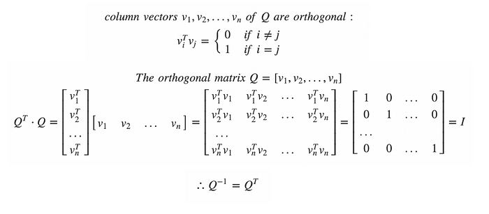
\] these vectors that make up \(\mathbf{X}\) are orthogonal (\(\mathbf{XX' = I}\)), which means that \(\mathbf{R = X \lambda X'}\)

For some demonstration in R, let’s create a correlation matrix

# lets create a correlation matrix, as f f'
f <- seq(.9,.4,-.1)
R <- f %*% t(f)
#give rownames and colnames
rownames(R)<-colnames(R)<-paste0("V",seq(1:6))
#constrain diagonals to equal 1
diag(R)<-1
# here's our correlation matrix!
R
     V1   V2   V3   V4   V5   V6
V1 1.00 0.72 0.63 0.54 0.45 0.36
V2 0.72 1.00 0.56 0.48 0.40 0.32
V3 0.63 0.56 1.00 0.42 0.35 0.28
V4 0.54 0.48 0.42 1.00 0.30 0.24
V5 0.45 0.40 0.35 0.30 1.00 0.20
V6 0.36 0.32 0.28 0.24 0.20 1.00

The actual solving of the eigen decomposition is too much for me, but luckily the function eigen() does it for us!

# do eigen decomposition
e <- eigen(R)
print(e, digits=2)
eigen() decomposition
$values
[1] 3.16 0.82 0.72 0.59 0.44 0.26

$vectors
      [,1]   [,2]   [,3]  [,4]   [,5]   [,6]
[1,] -0.50 -0.061  0.092  0.14  0.238  0.816
[2,] -0.47 -0.074  0.121  0.21  0.657 -0.533
[3,] -0.43 -0.096  0.182  0.53 -0.675 -0.184
[4,] -0.39 -0.142  0.414 -0.78 -0.201 -0.104
[5,] -0.34 -0.299 -0.860 -0.20 -0.108 -0.067
[6,] -0.28  0.934 -0.178 -0.10 -0.067 -0.045

It returns eigenvalues and corresponding eigenvectors.
The eigenvectors are orthogonal (\(\mathbf{XX' = I}\)):

round(e$vectors %*% t(e$vectors),2)
     [,1] [,2] [,3] [,4] [,5] [,6]
[1,]    1    0    0    0    0    0
[2,]    0    1    0    0    0    0
[3,]    0    0    1    0    0    0
[4,]    0    0    0    1    0    0
[5,]    0    0    0    0    1    0
[6,]    0    0    0    0    0    1

The eigenvectors represent the direction of the vectors, and the eigenvalues represent magnitude (i.e., how much variance of \(\mathbf{R}\) they capture).

Our Principal Components \(\mathbf{P}\) are the eigenvectors scaled by the square root of the eigenvalues:

# eigenvectors
# e$vectors
# scaled by sqrt of eigenvalues
# diag(sqrt(e$values))

P <- e$vectors %*% diag(sqrt(e$values))
P
           [,1]        [,2]       [,3]        [,4]        [,5]        [,6]
[1,] -0.8831928 -0.05536631  0.0782390  0.10701187  0.15835679  0.41743889
[2,] -0.8326442 -0.06733799  0.1025241  0.16479768  0.43606188 -0.27267156
[3,] -0.7697296 -0.08728107  0.1542466  0.40770515 -0.44832468 -0.09427542
[4,] -0.6937401 -0.12835669  0.3511553 -0.59865399 -0.13319887 -0.05301591
[5,] -0.6044520 -0.27121026 -0.7293067 -0.15137345 -0.07148043 -0.03422115
[6,] -0.5022823  0.84639719 -0.1512575 -0.07713676 -0.04428451 -0.02311401

$$ R = PP’

X

$$

And with all of them, we can perfectly reproduce our correlation matrix: \(\mathbf{R = PP'}\).

P %*% t(P)
     [,1] [,2] [,3] [,4] [,5] [,6]
[1,] 1.00 0.72 0.63 0.54 0.45 0.36
[2,] 0.72 1.00 0.56 0.48 0.40 0.32
[3,] 0.63 0.56 1.00 0.42 0.35 0.28
[4,] 0.54 0.48 0.42 1.00 0.30 0.24
[5,] 0.45 0.40 0.35 0.30 1.00 0.20
[6,] 0.36 0.32 0.28 0.24 0.20 1.00

But we don’t want to keep all of them, because then we are not reducing anything. So we might choose to keep, e.g., just one.

When “doing PCA” with the principal() function, we retain only one component with nfactors = 1:

library(psych)
pc1<-principal(R, nfactors = 1, covar = FALSE, rotate = 'none')
pc1
Principal Components Analysis
Call: principal(r = R, nfactors = 1, rotate = "none", covar = FALSE)
Standardized loadings (pattern matrix) based upon correlation matrix
    PC1   h2   u2 com
V1 0.88 0.78 0.22   1
V2 0.83 0.69 0.31   1
V3 0.77 0.59 0.41   1
V4 0.69 0.48 0.52   1
V5 0.60 0.37 0.63   1
V6 0.50 0.25 0.75   1

                PC1
SS loadings    3.16
Proportion Var 0.53

Mean item complexity =  1
Test of the hypothesis that 1 component is sufficient.

The root mean square of the residuals (RMSR) is  0.09 

Fit based upon off diagonal values = 0.95

Look familiar? It looks like the first component we computed manually. The first column of \(\mathbf{P}\). The direction is flipped, but that is somewhat irrelevant because it’s the same dimension (i.e., South is just “negative North”!)

cbind(pc1$loadings, P=P[,1])
         PC1          P
V1 0.8831928 -0.8831928
V2 0.8326442 -0.8326442
V3 0.7697296 -0.7697296
V4 0.6937401 -0.6937401
V5 0.6044520 -0.6044520
V6 0.5022823 -0.5022823

We can now ask “how well does this component (on its own) recreate our correlation matrix?”

P[,1] %*% t(P[,1])
          [,1]      [,2]      [,3]      [,4]      [,5]      [,6]
[1,] 0.7800296 0.7353854 0.6798197 0.6127063 0.5338477 0.4436121
[2,] 0.7353854 0.6932964 0.6409109 0.5776386 0.5032935 0.4182224
[3,] 0.6798197 0.6409109 0.5924836 0.5339923 0.4652646 0.3866215
[4,] 0.6127063 0.5776386 0.5339923 0.4812753 0.4193326 0.3484533
[5,] 0.5338477 0.5032935 0.4652646 0.4193326 0.3653623 0.3036056
[6,] 0.4436121 0.4182224 0.3866215 0.3484533 0.3036056 0.2522875

It looks close, but not quite. How much not quite? Measurably so!

R - (P[,1] %*% t(P[,1]))
            V1          V2          V3          V4          V5          V6
V1  0.21997041 -0.01538541 -0.04981966 -0.07270625 -0.08384772 -0.08361212
V2 -0.01538541  0.30670361 -0.08091089 -0.09763864 -0.10329350 -0.09822244
V3 -0.04981966 -0.08091089  0.40751635 -0.11399225 -0.11526463 -0.10662154
V4 -0.07270625 -0.09763864 -0.11399225  0.51872473 -0.11933260 -0.10845334
V5 -0.08384772 -0.10329350 -0.11526463 -0.11933260  0.63463772 -0.10360556
V6 -0.08361212 -0.09822244 -0.10662154 -0.10845334 -0.10360556  0.74771250

Notice the values on the diagonals of \(\mathbf{p_1}\mathbf{p_1}'\).

diag(P[,1] %*% t(P[,1]))
[1] 0.7800296 0.6932964 0.5924836 0.4812753 0.3653623 0.2522875

These aren’t 1, like they are in \(R\).
But they are proportional: this is the amount of variance in each observed variable that is explained by this first component.
The principal() function calls this ‘communalities’, which is really more of a term we see in factor analysis.

pc1$communality
       V1        V2        V3        V4        V5        V6 
0.7800296 0.6932964 0.5924836 0.4812753 0.3653623 0.2522875 

1 minus these values is the unexplained variance, or ‘uniqueness’:

1 - diag(P[,1] %*% t(P[,1]))
[1] 0.2199704 0.3067036 0.4075164 0.5187247 0.6346377 0.7477125
pc1$uniquenesses
       V1        V2        V3        V4        V5        V6 
0.2199704 0.3067036 0.4075164 0.5187247 0.6346377 0.7477125