8: Structural Equation Modelling

This reading:

• Combining a “measurement model” (see confirmatory factor analysis (CFA)) with a “structural model” (see path analysis), all at once — SEM!
  
• The process of doing SEM
• Other things we will need to bear in mind (normality of measured variables, categorical data, and missing data)

A unifying framework?

Let’s recap what we’ve seen so far.

In Chapters 1-4, we covered methods that moved from having many observed variables to being able to work with representations of the more abstract ideas that we are actually interested in. We introduced the idea of “latent variables” — variables that we cannot observe directly, but that we can posit as being the underlying cause of the covariance between the manifest “indicators” (the variables that we actually measure). We saw two methods for working with these latent variables (or “factors”): Exploratory and Confirmatory factor analysis (EFA and CFA). Broadly speaking, these two approaches worked towards different goals — we might use EFA to better understand the underlying number and correlations of the latent variables that underpin a set of indicators, and we would use CFA to assess an a priori (i.e., pre-specified) structure.

We then took a diversion into “path analysis” in Chapters 6-7. We learned how path analysis provides a method for estimating relationships in models where there can be multiple “endogenous” (think “outcomes”) variables. This could be contrasted with simpler regression models in which a set of variables are combine to predict a single outcome — in path analysis, the set of relationships between all variables in the system are used to imply a covariance matrix. This approach allows us to test theoretical models about a system of variables, or to estimate more complex paths in the system (such as in mediation analyses).

Throughout all these chapters we have started to do a lot of “thinking in diagrams”, where we draw out the different variables and the theorised paths between them. In the discussion of path analysis, however, we were only ever working with observed variables — our diagrams had only rectangles, and no circles/ovals.¹ But the assumption we were making, therefore, is that we are measuring everything perfectly — i.e., without error.

The natural question, therefore, is can we combine “path analysis” (testing theoretical models of relationships between variables) with the idea of “latent variables” (unobserved variables that directly represent the construct of interest, as measured by a set of indicators). And the answer is: Yes, we can! And it’s called “Structural Equation Modelling” (SEM).

SEM \(\ni\) path \(\ni\) lm \(\ni\) cor…

People love saying “your method is a special case of my method”.² Some might see our journey into statistics so far as:

• correlation and t-test are just special cases of a linear model, where there is a single predictor (correlation = lm with a continuous predictor, t.test = lm with a binary predictor)
• a linear model is just a special case of a path model, where there is only one endogenous variable
• a path model is just a special case of a structural equation model, where there are no latent variables

Structural Equation Modelling (SEM)

As we have already seen confirmatory factor analysis (CFA) and path analysis, we actually don’t have to cover anything new in order to get to Structural Equation Modelling (SEM).

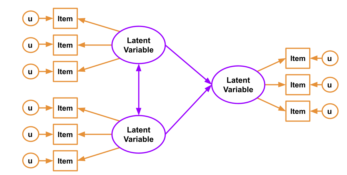
Path analysis, as we saw in Chapter 6, offers a way of specifying and evaluating a structural model, in which variables relate to one another in various ways, via different (sometimes indirect) paths. Factor Analysis, on the other hand, brings something absolutely crucial to the table — a measurement model. Factor analysis allows us to mitigate some of the problems which are associated with measurement error by specifying the existence of some latent variable which is measured via our observed variables. No question can perfectly measure someone’s level of “anxiety”, but if we take a set of 10 carefully chosen questions, we can consider the shared covariance between those 10 questions to represent the construct that is common between all of them (they all ask, in different ways, about “anxiety”), also modeling the unique error with which each individual question fails to perfectly represent the entire construct.

In SEM, we just combine these two parts! We have both a structural model and a measurement model. The measurement model is our specification between the items we directly observed, and the latent variables of which we consider these items to be manifestations. The structural model is our specified model of the relationships between the things we’re interested in (the latent variables, along with other variables that might f).

Figure 1: SEM diagram. Measurement model in orange, Structural model in purple

Why bother?

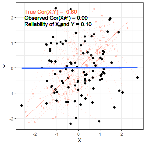
The worse a variable is at measuring a construct, the harder it is for us to gain anything meaningful from that variable. To take this to the extreme, suppose that we wanted to estimate cor(height, age) and instead of recording age accurately, we just filled it the variable with completely random numbers — would we see a positive correlation? probably not!

The animation below shows this idea. It shows two variables X and Y, that have a correlation of 0.8. This is the correlation we would observe if we could measure them perfectly. But we can never measure things perfectly! The more measurement error that we add, the more the correlation we observe goes towards zero. This will happens as measurement error increases on either variable (or both, as in the animation!)

SEM explicitly incorporates measurement error into the model, allowing us to estimate more accurately the associations between the things we’re actually interested in (the unobserved constructs).

Figure 2: The estimated correlation between two variables will decrease as the amount of measurement error increases.

SEM in R with lavaan

In R, we can fit SEM with the lavaan package in much the same way as we might fit CFA or path models. First we specify the model formula as a big long character string (we can include comments in here too):

mod <- "
  # measurement model
  F1 =~ y1 + y2 + y3 + y4
  F2 =~ y5 + y6 + y7 
  F3 =~ y8 + y9 + y10
  
  # structural part
  F1 ~ F2 + F3
"

Then we fit the model to the data:

mod.est <- sem(mod, data)

And then examine the fitted model using all the same functions we have already seen:

function	usage
summary(mod.est, ...)   standardized = TRUE     adds standardised estimates   ci = TRUE     adds confidence intervals   fitmeasures = TRUE     shows common fit metrics at the top	outputs the estimates for all model parameters (split into factor loadings, regressions, covariances, variances/residual variances, and defined parameters). Each parameter is presented with the associated standard error, z-statistic and p-value.
fitmeasures(mod.est)	Outputs many measures of model fit (see Chapter 4). These are a named list of numbers, so if we want to see just the more commonly used metrics, we can do: fitmeasures(mod.est)[c("rmsea","srmr","tli","cfi")]
parameterestimates(mod.est)	Outputs a neat table of all the parameter estimates, along with standard errors, z-statistics, p-values and confidence intervals
standardizedsolution(mod.est)	Outputs a neat table of standardised estimates and significance tests and confidence intervals for these standardised estimates.3

The six steps of SEM?

There are quite a lot of books, papers, tutorials and resources that tend to present SEM as a step-by-step procedure. These are generally something along the lines of:

1. assumptions, measures, data
   1. check for (non-)normality of items (more on this below)
   2. assess the measurement model
2. specification
   1. draw out your model
   2. write your model formula
3. identification & estimation
   1. essentially “fit the model”, using an appropriate estimator (more on this below)
4. evaluation
   1. examine model fit (see Chapter 4#model-fit).
5. re-specification
   1. modify your model (see Chapter 4#model-modifications).
6. interpretation
   1. depending on the research aims, interpretation will often be focused on the paths in the structural part of the model

Note that step 1 is very important. If you test the relationships between a set of latent factors, and they are not reliably measured by the observed items, then this error propagates up to influence the fit of the structural model.

To test the measurement model, it is typical to fit individual CFA models for each construct and assess their fit (making any reasonable adjustments if necessary) prior to then fitting the full SEM. An alternative approach is to saturate the structural model (i.e., allow all the latent variables to correlate with one another), meaning any misfit is due to the measurement model only.

You can’t test the structural model if the measurement model is bad

Additional considerations

Non-normality

One of the key assumptions of the models we have been fitting so far is that our variables are all normally distributed, and are continuous. Why?

Recall that all of these covariance-based models (path analysis, CFA, SEM) involve comparing the observed covariance matrix with our model implied covariance matrix. This heavily relies on the assumption that our observed covariance matrix provides a good representation of our data - i.e., that \(var(y_i)\) and \(cov(y_i,y_j)\) are adequate representations of the relations between variables. While this is true if we have a “multivariate normal distribution”, things become more difficult when our variables are either not continuous or not normally distributed.

The multivariate normal distribution is fundamentally just the extension of our univariate normal (the bell-shaped curve we are used to seeing) to more dimensions. The condition which needs to be met is that every linear combination of the \(k\) variables has a univariate normal distribution. It is denoted by \(\sim N(\boldsymbol{\mu}, \boldsymbol{\Sigma})\) (note that the bold font indicates that \(\boldsymbol{\mu}\) and \(\boldsymbol{\Sigma}\) are, respectively, a vector of means and a matrix of covariances).⁴

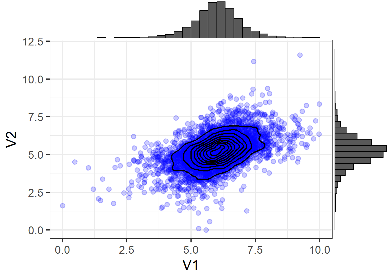
The idea of the multivariate normal can be a bit difficult to get to grips with in part because there’s not an intuitive way to visualise it once we move beyond 2 or 3 variables. With 2 variables, you can think of it just like a density plot but in 3 dimensions, as in Figure 3 and Figure 5. You can also represent these as “contour” plots (Figure 4,Figure 6), which is like looking down on the 3D plots from above (just like a map!)

3D (Normal)

Figure 3: Bivariate Normal

Contour (Normal)

Figure 4: Contour plot for a normal bivariate distribution. Marginal distributions of each variable are presented along each axis

3D (Non-Normal)

Figure 5: Bivariate distribution of some skewed variables

Contour (Non-Normal)

Figure 6: Contour plot for a non-normal bivariate distribution. Marginal distributions of each variable are presented along each axis

Using means and covariances to summarise a distribution means we are capturing two features of the distribution: location and scale (the mean moves the center of a distribution up and down a number line, and the variance and covariance captures the spread and relationships between variables).

There are two more, “skewness” and “kurtosis” which are rarely the focus of investigation (the questions we ask tend to be mainly concerned with means and variances). Skewness is a measure of asymmetry in a distribution. Distributions can be positively skewed or negatively skewed, and this influences our measures of central tendency and of spread to different degrees. The kurtosis is a measure of how “pointy” vs “rounded” the shape of a distribution is.

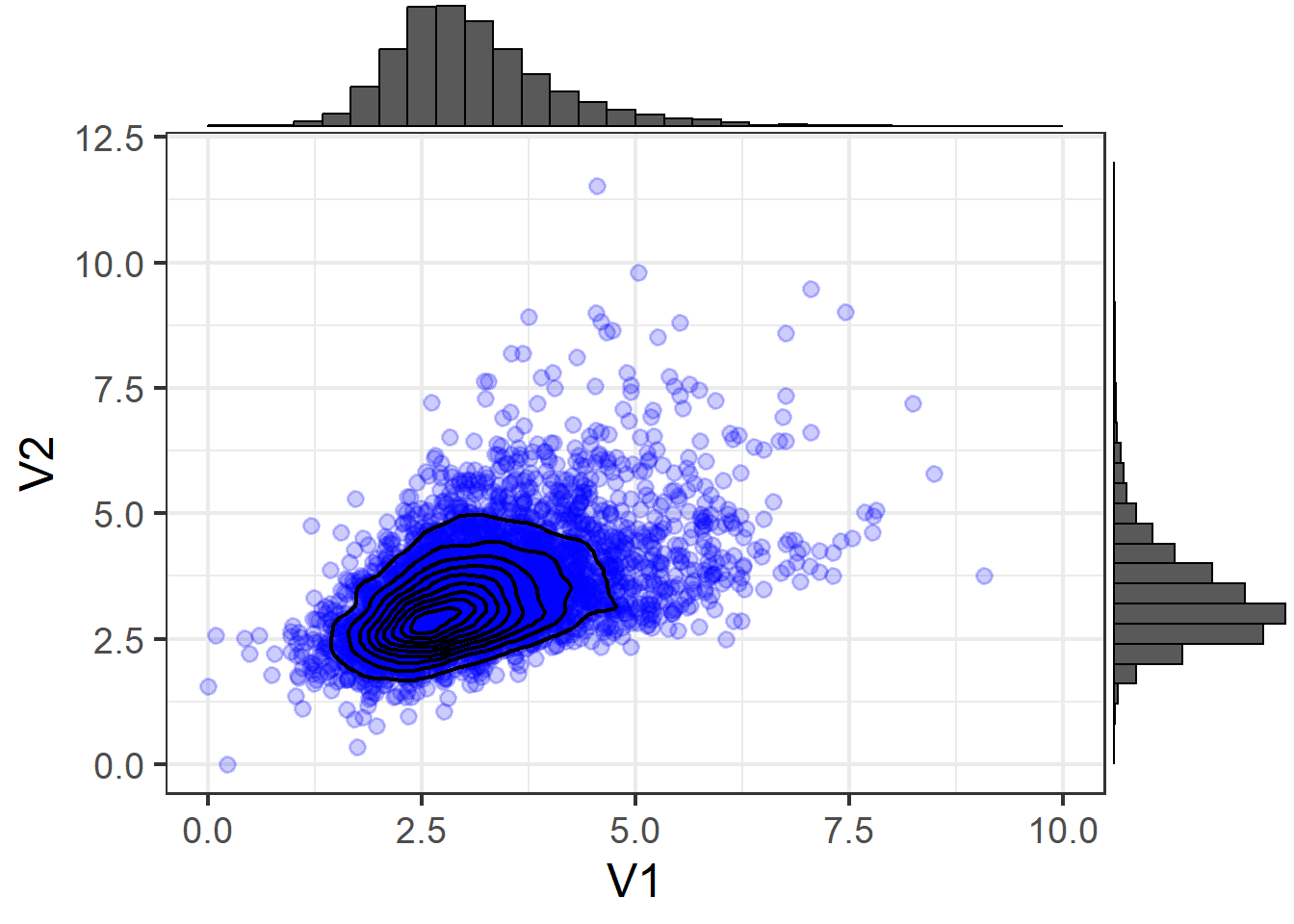
Note that in Figure 5 and Figure 6, the distribution is exhibiting some skew! If we have variables that look like this as part of our SEM, we need to be careful, because we will be trying to capture the pattern with means and covariances.

optional: demonstration

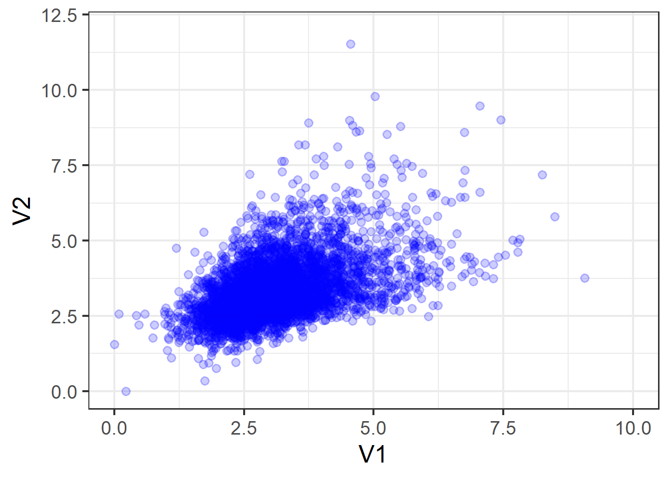
If we take the two variables shown in the figure below and try to summarise them using mean and covariances:

The data:

the means:

      V1       V2 
3.114552 3.354231 

the covariance matrix:

          V1        V2
V1 0.9561678 0.4874602
V2 0.4874602 0.9837609

But this fails to capture information about important properties of the data relating to features such as skew (lop-sided-ness) and kurtosis (pointiness).

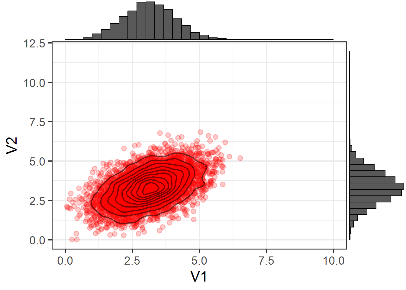
To demonstrate, suppose we were to take these means and covariances, and simulate some new data based on these numbers. This would, essentially be randomly sampling data from the multivariate normal distribution:

\[ \sim N \left( \begin{bmatrix} 3.12 \\ 3.35 \end{bmatrix}, \begin{bmatrix} 0.96 & 0.49 \\ 0.49 & 0.98 \end{bmatrix} \right) \]

We would get something like Figure 7, which is clearly not a very good representation of our actual data.

Figure 7: Data simulated from means and covariances. Even if the original variables are skewed, the means and covariances contain information on only 2 ‘moments’ of the variables: their scale (spread) and location (center).

For determining what constitutes deviations from normality, there are various ways to calculate the skewness and kurtosis of univariate distributions.⁵ In addition, there are various suggested rules of thumb we can follow. Below are the most common:

Skewness rules of thumb:

• \(|skew| < 0.5\): fairly symmetrical
• \(0.5 < |skew| < 1\): moderately skewed
• \(1 < |skew|\): highly skewed

Kurtosis rule of thumb:

• \(Kurtosis > 3\): Heavier tails than the normal distribution. Possibly problematic

How can we check?

We really want to be able to examine the multivariate normality, but more often than not, we just look at the normality of each variable separately.

To do so, we can:

• The multi.hist() function from the psych package is very handy here. E.g., using data |> select(var1, var2, ...) |> multi.hist() will quickly plot histograms for all our selected variables, along with normal curves imposed to get a sense of how far off our assumptions are.
• The describe() function from the psych package will provide measures of both skew and kurtosis.

optional: we can still be tricked!

Even if each variable looks normally distributed when we plot it on its own, this doesn’t mean the joint distribution is normal!

A bivariate distribution that is not-normal, but for which marginal distributions of both variables are normal

What can we do?

In the event of non-normality, we can still use maximum likelihood to find our estimated factor loadings, coefficients and covariances. However, our standard errors (and our \(\chi^2\) model fit) will be biased. We can use a robust maximum likelihood estimator that essentially applies corrections to the standard errors⁶ and \(\chi^2\) statistic.

There are a few robust estimators in lavaan, but one of the more frequently used ones is “MLR” (maximum likelihood with robust SEs). You can find all the other options at https://lavaan.ugent.be/tutorial/est.html.
We can make use of these estimators⁷ with:

sem(model, estimator="MLR")

When we use these estimators, we will often be able to get out “robust” versions of the model fit statistics. summary(model, fitmeasures = TRUE) will print these out alongside the standard metrics, or we can ask for them specifically:

fitmeasures(model)[c("rmsea.robust","srmr","cfi.robust","tli.robust")]

Categorical variables

So far in our discussion of factor analysis, path analysis and structural equation modelling, we have been working only with continuous variables (or variables that we have been treating as if they were continuous!).

We can use categorical variables in these models, but how we treat them depends on whether they are exogenous (only arrows coming out) or endogenous (arrows going in).

Exogenous categorical variables

Remember that in the linear regression world, when we have a categorical predictor in the model, then we end up estimating a set of “contrasts” — i.e., differences in the outcome between the levels of the predictor. If our categorical predictor has \(k\) levels to it, then we get out \(k-1\) coefficients.

In path analytic models, categorical variables present a challenge because there is not one single coefficient for a path from predictor to outcome.

There are a few options for us here:

1. if the predictor is binary, then just set the values to 0 and 1
2. if the predictor has \(k\) levels, then manually create a set of \(k-1\) dummy variables and enter those into the model
   
3. if the predictor is ordinal, then use numeric values. The downside here is that it assumes equal distance between the levels.

Endogenous categorical variables

If we have endogenous variables that are categorical, then things become a bit more tricky.

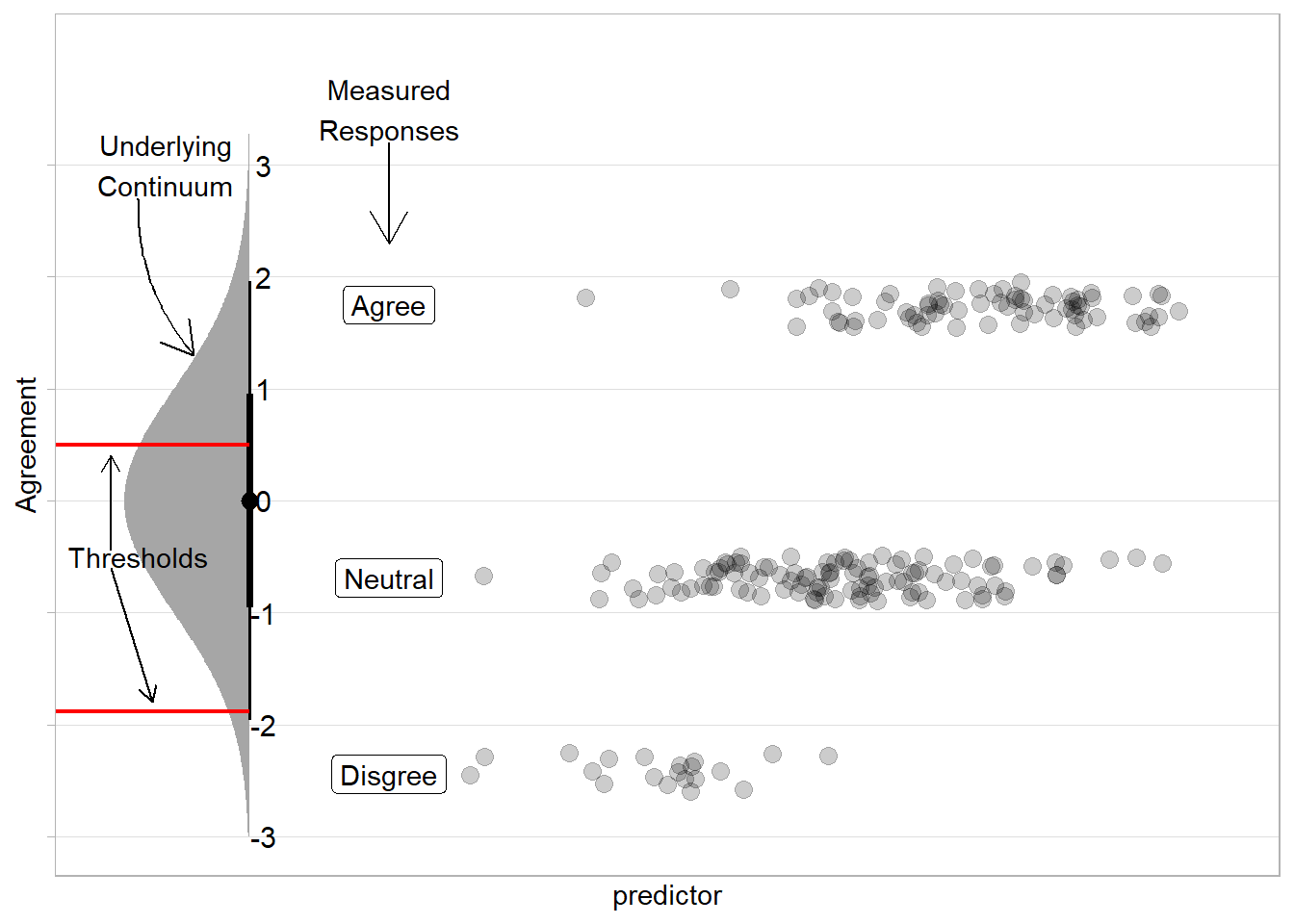
This might be a far more common problem than you might think! Remember that if we are using a variable as an indicator of a latent factor, then it is endogenous, and think about how we tend to set up questionnaires - we use Likert scales that ask people to rate agreement with statements, and people choose from “Strongly Disagree”, …. , to “Strongly Agree”.

These response options are not on a continuous scale, yet we often pretend that they are! We convert them to numbers from 1 to 5, and then go ahead with our modelling.

This is a contentious issue: some statisticians might maintain that it is never appropriate to treat ordinal data as continuous. Others feel that it’s generally okay — an often used rule of thumb is that Likert data with \(\geq 5\) levels can be treated as if they are continuous without unduly influencing results.⁸

But what if we don’t have 5+ levels? Or we just don’t want to assume Likert data is continuous? An important note is that even if our questionnaire included 5 response options for people to choose from, if participants only used 3 of them, then we would actually have a variable with just 3 levels.

Estimation techniques exist that allow us to model such variables by considering the set of ordered responses to correspond to portions of an underlying continuum. This involves estimating the ‘thresholds’ of that underlying distribution at which people switch from giving one response to the next.

The intuition to this is to imagine a distribution that represents the unmeasured continuum — so if we are measuring agreement with a statement, but we have only the options “disagree”,“neutral”,“agree”, then these options will represents sections of a continuous distribution of “agreement”. If we had the same number of responses to each option (e.g., 30 “disagree”, 30 “neutral”, and 30 “agree”) then we would split the distribution into equal thirds. A predictor’s coefficient shifts this underlying distribution, essentially adjusting the probability of responses falling into each category based on value of the predictor.

Figure 8: modelling ordinal outcomes typically involves modelling ‘thresholds’ (cut-points) on an underlying continuum

What can we do?

In R, lavaan will automatically switch to an appropriate estimator for categorical variables (called “DWLS”⁹) if we tell it that we have some ordered-categorical variables:¹⁰

sem(model, 
    ordered = c("item1","item2","item3", ...))

Or if all of our endogenous variables are categorical, we can simply use:

sem(model, 
    ordered = TRUE)

Although very rarely of interest to us, the resulting models will also print out the set of estimated thresholds (along with the loadings, regressions, covariances, residual variances etc). For each variable, if there are \(k\) levels to the response scale, then there will be \(k-1\) estimated thresholds in the output.

Missing data

It is very common to have missing data. Participants may stop halfway through the study, may decline to be followed up (if it is longitudinal) or may simply decline to answer certain sections. In addition, missing data can occur for all sorts of technical reasons (e.g, website crash and auto-submit a questionnaire, etc.).

It is important to understand the possible reasons for missing data in order to appropriately consider what data you do have. If missing data are missing completely random, then the data you do have should still be representative of the population. But suppose you are studying cognitive decline in an aging population, and people who are suffering from cognitive impairment are less likely to attend the follow-up assessments. Is this missingness random? No. Does it affect how you should consider your available data to represent the population of interest? Yes.

There are three main reasons that we certain data may be missing, and the acronyms are a nightmare:¹¹

• MCAR: Missing Completely At Random. Data which are MCAR are missing data for which the propensity for missingness is completely independent of any observed or unobserved variables. It is truly random if the data are missing or not.

• MAR: Missing At Random. Data which are MAR are missing data for which the propensity for missingness can be fully explained by some other variables for which there are measurements. In other words, there is a systematic relationship between missing values and observed values. For example, people who are unemployed at time of assessment will likely not respond to questions on work-life satisfaction. If we have also measured employment status then the missing values of work-life satisfaction can be explained by the observed values of employment status.

• MNAR: Missing Not At Random. Data which are MNAR are missing data for which the propensity for missingness is related to the value which is missing. For example, suppose an employer tells employees that there are a limited number of bonuses to hand out, and then employees are asked to fill out a questionnaire. Those who are less satisfied with their job may not respond to questions on job satisfaction (if they believe it will negatively impact their chances of receiving a bonus).

What can we do?

In SEM, there is an extremely useful method known as full information maximum likelihood (FIML) which, allows us to use all our available data (including those that have only some values present).

FIML separates data into the different patterns of missingness (i.e. those that are missing on IQ1, those missing on IQ1 and IQ2, those missing on just IQ2, and so on). The likelihood (“probability of seeing this data given these parameters”) of each group can be estimated from the parameters that are available for that pattern. The estimation process then finds the set of parameters that maximise the likelihood of the full dataset (we can combine likelihoods of the datasets with each missingness pattern). This way it utilises all observed variables (hence “full information”) to estimate the model parameters.

A downside, one could argue, is that you may have specific theoretical considerations about which observed variables should weigh in on estimating missingness in variable \(x\) (rather than all variables), in which case imputation techniques may be preferable. FIML only provides unbiased estimates if the data are MAR (i.e. if the missingness depends on other variables present in the data).

In lavaan, we can make use of full information maximum likelihood by using either missing = "FIML" or missing = "ML" (they’re the same) in the functions cfa() and sem().

optional: other approaches to missingness

Thus far in our analyses, we have been simply excluding any row for which there is missingness. This is typically known as “listwise deletion”, and is the default for many modelling approaches. Any person who is missing some data on a variable in our model will simply not be included. This method assumes that the data are “Missing Completely At Random”, because we make the assumption that studying only the people who have complete data does not bias our results in any way.

Other traditional approaches are to use basic imputation methods such as “mean/median imputation” (replace missing values with the average of that variable). These can be okay, but they assume that the imputed values are exactly what we would have observed had it not been missing, rather than estimates. The lack of variability around this imputed value will shrink the standard errors because it is assumed that no deviations exist among the substituted values.

Another option is “regression imputation”, where we replace missing values with the predicted values from a regression model of the variable with missingness onto some relevant predictors. This is better because our estimates of the values of missing observations could be much better, but we still make an assumption that these estimates are perfect, when we know they are just estimates.

A more sophisticated approach to this is “Multiple Imputation” (MI). Multiple imputation is similar to the regression imputation approach described above in that it predicts the value of missing observations based on the covariates, but instead of predicting just one value, it predicts many. Rather than saying “the predicted value for this missing observation is 5”, we say “the predicted value for this missing observation is from the distribution \(\sim N(5,2)\)”. So we simulate \(m\) draws from that distribution, and we end up with \(m\) predicted values. We make \(m\) copies of our data and replace the missing observations with each of our \(m\) predicted values. We then do our analysis on each \(m\) imputed dataset, and pool the results!

Footnotes

1. with the exception of residuals, which are always unobserved latent variables!

2. the \(\ni\) symbol in \(A \ni x\) just means \(A\) contains \(x\)

3. It’s tempting to expect the z-statistics to be the same for standardised/unstandardised estimates, but they won’t be.
   Back in the regression world, standardised and unstandardised coefficients have the same test statistic (\(t\), \(z\), whatever we’re using), because when we standardise we treat the observed sample variances as fixed things, and we just do \(\beta_{std} = b_{unstd} \times \frac{SD_x}{SD_y}\). The standard errors for the \(b_{unstd}\) undergoes the same calculation to get the standard error for \(\beta_{std}\), meaning the test statistic doesn’t change because the both estimate and standard error are just being multiplied by a constant (\(\frac{SD_x}{SD_y}\)), so \(\frac{b}{SE_b} = \frac{\beta}{SE_\beta}\).
   In SEM, however, the variances/SDs of x and y are part of the model, and these themselves have standard errors too! So the uncertainty in \(SD_x\) and \(SD_y\) get incorporated into the standardisation, changing the resulting test statistic!

4. We’ve actually seen this previously in multilevel modelling, when we had random intercepts, random slopes, and the covariance between the two!

5. (see Joanes, D.N. and Gill, C.A (1998). Comparing measures of sample skewness and kurtosis if you’re interested)

6. These are similar corrections to ones that we apply in a regression world, see LM Troubleshooting

7. (also works with the cfa() function)

8. see Johnson, D.R., & Creech, J.C. (1983). Ordinal measures in multiple indicator models: A simulation study of categorization error

9. Diagonally Weighted Least Squares

10. (also works with the cfa() function)

11. To me, these are some of the most confusing terms in statistics, because “at random” is used to mean “not completely random”!?? It might be easier to think of “missing at random” as “missing conditionally at random”, but then it gives the same acronym as “completely at random”!