| Variable | Description |
|---|---|
| type | College Type: −1 = Not reported; 1 = Public; 2 = Private for-profit; 3 = Private not-for-profit (no religious affiliation); 4 = Private not-for-profit (religious affiliation) |
| region | Region: 0 = US Service schools; 1 = New England; 2 = Mid East; 3 = Great Lakes; 4 = Plains; 5 = Southeast; 6 = Southwest; 7 = Rocky Mountains; 8 = Far West; 9 = Outlying areas |
| gradrate | Graduation Rate – All NA = missing |
| gradratem | Graduation Rate – Men NA = missing |
| gradratew | Graduation Rate – Women NA = missing |
Confidence intervals
Semester 2 - Week 1
1 Formative report C
Download the template Rmd file and start your work there. Save your work regularly by clicking File > Save.
Instructions - Don’t Skip!
Formative Report C covers the labs from weeks 1-5 of the DAPR1 course in semester 2. You’ll need to create a PDF report using RMarkdown, which will be submitted by 12 noon on Friday, 14th February 2025. Remember, these submissions are group-based, so there are no extensions. Expect written formative feedback in flexible learning week.
Your report should be tailored for a reader with basic statistical knowledge and should not include any references to R code or functions in the main report write-up. Instead, keep the main report focused on text, figures, and tables. All R code should be included in the compulsory Appendix B for reproducibility, which is automatically created for you in the template Rmd file. If you need to add extra tables or figures that don’t fit in the main part of the report, you can use an optional Appendix A. Remember, the main report should be a PDF file and should not exceed six sides of A4 paper, though appendices at the end don’t count towards this limit.
Ensure to use the default settings for font and page margins in your RMarkdown file. Also, make sure your report title includes your group name: Group NAME.LETTER, and list the exam numbers of all group members in the author section.
Don’t forget to register for your lab table group on LEARN by navigating to the course LEARN page, clicking on Groups, selecting Labs_1_2_3, finding your group, and clicking Join.
Formatting resources
At this page you can find resources to help you with your report formatting.
1.1 Data and Goal
In this report, to be done over weeks 1-5, you will estimate the mean graduation rate of female students in US colleges and universities in 2012, and test whether this value differs from a baseline rate of 50%. To do so, you will be using the dataset ipeds-2012.csv, available at https://uoepsy.github.io/data/ipeds-2012.csv. This is a subset of data derived from the 2012 Integrated Postsecondary Education Data System (IPEDS) at the National Center for Education Statistics, and gives you experience of working with governmental data. The data were collected for a random sample from all colleges and universities in the United States in that year.
In the US, a university is typically a larger institution offering both undergraduate and graduate degrees with a research focus, while a college is typically an institution of moderate/smaller size and primarily providing undergraduate education. The terms are often used interchangeably, but universities tend to be more comprehensive in their academic offerings and scale.
The variables include:
1.2 This week’s task
Task C1
Read the data into R, describe the variable of interest both visually and numerically, and provide an estimate and 95% CI for the mean graduation rate of female students at US colleges and universities in 2012.
Sub-steps
Below there are sub-steps you need to consider to complete this week’s task.
Tip
To see the hints, hover your cursor on the superscript numbers.
-
Read the data into R and inspect it.1
- How many units are there?
- What’s the type of each variable?
- Are there any missing values in some variables? What about in the variable of interest for your analysis?
Visualise the distribution of the variable of interest (
gradratew). What is the shape of the distribution? Are there any outliers?2Compute and interpret a table of descriptive statistics for the variable of interest. At a minimum, ensure that it includes both a measure of centre and spread.3
Compute a 95% confidence interval for the mean graduation rate of female college students in 2012.4
For the report introduction, write a brief introduction to the data and question being investigated. How many cases are there? Are there any impossible or missing values? What is the type of the variables and which one is used for the investigation?
Provide a write up of your results so far, using proper rounding and making sure to report your results in context of the investigation.
2 Worked Example
The Procrastination Assessment Scale for Students (PASS) was designed to assess how individuals approach decision situations, specifically the tendency of individuals to postpone decisions (Solomon & Rothblum, 1984).
The PASS assesses the prevalence of procrastination in six areas: writing a paper; studying for an exam; keeping up with reading; administrative tasks; attending meetings; and performing general tasks. For a measure of total endorsement of procrastination, responses to 18 questions (each measured on a 1-5 scale) are summed together, providing a single score for each participant (range 0 to 90). The mean score from Solomon & Rothblum, 1984 was 33.
Investigation:
What is the average procrastination score of Edinburgh University students?
To answer this question, we will use data collected for a random sample of students from the University of Edinburgh: https://uoepsy.github.io/data/pass_scores.csv
| Variable Name | Description |
|---|---|
| sid | Subject identifier |
| school | School each subject belonged to |
| PASS | Total endorsement of procrastination score |
Necessary packages:
- tidyverse for using
read_csv(), usingsummarise()andggplot(). - patchwork for arranging plots side by side or underneath
- kableExtra for creating user-friendly tables
Read the data into R:
To inspect the data:
head(pass_scores)# A tibble: 6 × 3
sid school PASS
<chr> <chr> <dbl>
1 s_1 GeoSciences 31
2 s_2 ECA 24
3 s_3 LAW 32
4 s_4 ECA 40
5 s_5 LAW 28
6 s_6 SSPS 31glimpse(pass_scores)Rows: 20
Columns: 3
$ sid <chr> "s_1", "s_2", "s_3", "s_4", "s_5", "s_6", "s_7", "s_8", "s_9", …
$ school <chr> "GeoSciences", "ECA", "LAW", "ECA", "LAW", "SSPS", "PPLS", "SLL…
$ PASS <dbl> 31, 24, 32, 40, 28, 31, 30, 28, 32, 29, 28, 33, 35, 33, 30, 31,…summary(pass_scores) sid school PASS
Length:20 Length:20 Min. :24.00
Class :character Class :character 1st Qu.:28.75
Mode :character Mode :character Median :31.00
Mean :30.70
3rd Qu.:32.00
Max. :40.00 Visualise the distribution of PASS scores:
Note
The boxplot highlights an outlier (40). However, this value is well within the plausible range of the scale (0 – 90), hence it is of no concern and the point can be kept for the analysis.
plt_hist <- ggplot(pass_scores, aes(x = PASS)) +
    geom_histogram(color = 'white')

plt_box <- ggplot(pass_scores, aes(x = PASS)) +
    geom_boxplot()

plt_hist / plt_box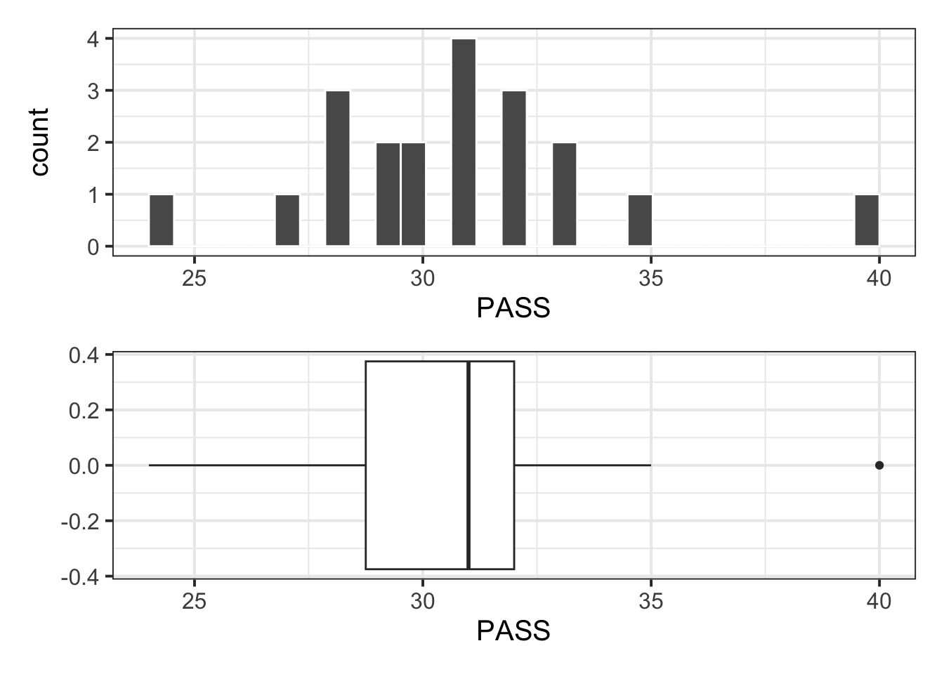
Descriptive statistics:
stats |>
    kbl(booktabs = TRUE, digits = 2,
caption = "Descriptive statistics for PASS scores")| n | Min | Max | M | SD |
|---|---|---|---|---|
| 20 | 24 | 40 | 30.7 | 3.31 |
When estimating a parameter, in this case the mean score on the Procrastination Assessment Scale for Students (PASS) for all Edinburgh University students, we do not just report the estimate (sample average score), but also something that reflects our uncertainty in the estimate. This can either be the standard error or a confidence interval. If asked to compute a 95% confidence interval for the mean score on the Procrastination Assessment Scale for Students (PASS) for all Edinburgh University students, we could do:
# Sample mean
xbar <- stats$M

# Standard error
s <- stats$SD
n <- stats$n
se <- s / sqrt(n)
se
[1] 0.7401991[1] -2.093024 2.093024# CI
xbar + tstar * se[1] 29.15075 32.24925WARNING!
This code won’t work if stats stores a kable, i.e. the result of kbl(). Make sure this only stores the tibble, rather than the pretty version from kbl()!
Reporting
These three code chunks should not be visible in the report. You can simply report the CI in a paragraph using the style [LowerCI, UpperCI].
Example introduction
A random sample of 20 students from the University of Edinburgh completed a questionnaire measuring their total endorsement of procrastination. The data, available from https://uoepsy.github.io/data/pass_scores.csv, were used to estimate the average procrastination score of all Edinburgh University students. The recorded variables included a subject identifier (sid), the school of each subject (school), and the total score on the Procrastination Assessment Scale for Students (PASS). The data do not include any impossible values for the PASS scores, as they were all within the possible range of 0 – 90. To answer the question of interest, in the following we will only focus on the total PASS score variable.
Example CI interpretation
From the sample data we obtain an average procrastination score of \(M = 30.7\), 95% CI [29.15, 32.25]. Hence, we are 95% confident that a Edinburgh University student will have a procrastination score between 29.15 and 32.25, which is between 0.75 and 3.85 lower than the average score of 33 reported by Solomon & Rothblum.
3 Student Glossary
To conclude the lab, add the new functions to the glossary of R functions.
| Function | (package) and use |
|---|---|
geom_histogram |
(tidyverse) creates a histogram |
geom_boxplot |
(tidyverse) creates a boxplot |
summarise |
(tidyverse) compute a numerical summary of the data |
n() |
(tidyverse) count the rows. To be used inside summarise()
|
mean |
Compute the mean of a column |
sd |
Compute the standard deviation of a column |
qt |
Computes the quantile of a t distribution. For example, qt(0.1, df = 21) returns the value in a t(21) distribution that cuts a probability of 0.1 to its left |
Footnotes
Hint: Some of the following functions may be useful:
read_csv()from tidyverse,head(),glimpse(),summary(),nrow(DATA),dim(DATA),length(DATA$VARIABLE),DATA |> summarise(n = n())↩︎Hint:
geom_histogram(),geom_density(),geom_boxplot()may be useful functions.
To get rid of NAs in a variable of interest, you can useDATA |> drop_na(VARIABLE)or addna.rmas an argument tomean(),sd(), etc.
We don’t recommend usingna.omit()on the entire dataset, as it would remove any row with NAs, even in variables not used for the current analysis.↩︎Hint:
summarise()from the tidyverse package ordescribe()from the psych package↩︎-
Hints:
Step 1: Compute the average gradution rate of female college students
Step 2: Compute the standard error of the mean
Step 3: Compute the quantiles of a t distribution with \(n-1\) degrees of freedom, where \(n\) = sample size, cutting a probability of 0.95 in between them.
Step 4: Obtain the confidence interval using the formula:
\[95\% \text{ CI: } \left[ \bar x - t^* \ SE_{\bar{x}}, \ \bar x + t^* \ SE_{\bar{x}} \right]\] \[\text{where} \qquad SE_{\bar{x}} = \frac{s}{\sqrt n}\]↩︎