Key question
Can we trust self-reported voting turnout?
Consider the data stored in the file turnout.csv. These represent measurements on US election turnout data and will be used to investigate whether there is a bias in self-reported voting turnout. In a nutshell, people are becoming more concerned about accuracy of answers to post-election surveys as people might lie about about whether or not they voted due to social desirability bias. Perhaps the respondent felt like they should have voted when in fact they didn’t vote. You will investigate whether this sort of bias is present in the survey conducted by the American National Election Studies (ANES).
| Variable | Description |
|---|---|
| year | election year |
| ANES | ANES estimated turnout rate |
| VEP | voting eligible population (in thousands) |
| VAP | voting age population (in thousands) |
| total | total ballots cast for highest office (in thousands) |
| felons | total ineligible felons (in thousands) |
| noncitizens | total noncitizens (in thousands) |
| overseas | total eligible overseas voters (in thousands) |
| osvoters | total ballots counted by overseas voters (in thousands) |
How do we measure turnout rates? The numerator should be the total votes that were cast, while we have two choices for the denominator:
- Registered voters
- VAP (voting-age population) from Census
- VEP (voting-eligible population)
Both VAP and VEP do not count overseas voters, so if those data are available we may want to use it. Furthermore, we have that
\[ \text{VEP = VAP + overseas voters} - \text{ineligible voters} \]
where:
- overseas voters: military personnel and civilians
- ineligible voters: non-citizens, disenfranchised felons, those who failed to meet states’ residency requirement, etc.
Q1
Exercise
Read the data into R.
How many variables and observations are there?
What’s the range of years covered by this survey?
Answer
# A tibble: 6 x 9
   year    VEP    VAP total  ANES felons noncit overseas osvoters
  <dbl>  <dbl>  <dbl> <dbl> <dbl>  <dbl>  <dbl>    <dbl>    <dbl>
1  1980 159635 164445 86515    71    802   5756     1803       NA
2  1982 160467 166028 67616    60    960   6641     1982       NA
3  1984 167702 173995 92653    74   1165   7482     2361       NA
4  1986 170396 177922 64991    53   1367   8362     2216       NA
5  1988 173579 181955 91595    70   1594   9280     2257       NA
6 1990 176629 186159 67859 47 1901 10239 2659 NAdim(turnout)
[1] 14 9range(turnout$year)
[1] 1980 2008The file stores measurements on 9 variables for 14 years. The range of years covered by the ANES survey is 1980 to 2008.
Q2
Exercise
Adjust the voting age population (VAP) to also include overseas voters.
Using the adjusted VAP, calculate the turnout rate. Finally, calculate the turnout rate using the voting eligible population (VEP) as the denominator. What differences do you observe?
Answer
turnout$ANES
[1] 71 60 74 53 70 47 75 56 73 52 73 62 77 78The ANES estimated turnout rate is out of 100, so we will express rates as percentages instead of proportions.
turnout$VAPtr <- turnout$total / (turnout$VAP + turnout$overseas) * 100
turnout$VEPtr <- turnout$total / turnout$VEP * 100
turnout$VEPtr - turnout$VAPtr
 [1] 2.155785 1.891789 2.711115 2.062703 3.045878 2.480105 4.072866
[8] 3.095397 4.124166 3.261470 4.882388 3.682145 5.553078 5.880239ggplot(turnout) +
geom_line(aes(year, VAPtr)) +
geom_point(aes(year, VAPtr)) +
geom_line(aes(year, VEPtr), color = 'red', linetype = 2) +
geom_point(aes(year, VEPtr), color = 'red', linetype = 2) +
labs(x = 'Year', y = 'Turnout rate (black: VAP, red: VEP)')
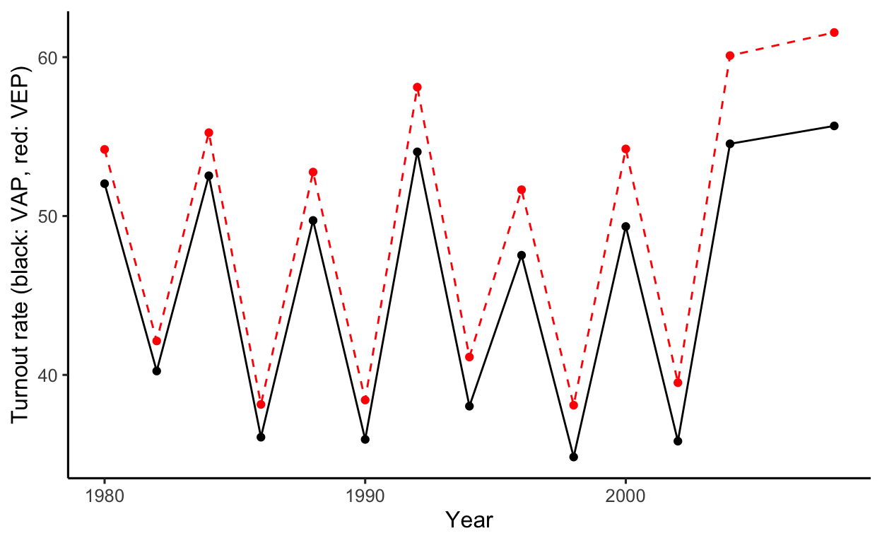
It appears that the estimated turnout rate based on the VAP is always lower than the estimate using the VEP.
Q3
Exercise
Calculate the bias between the ANES estimate of the turnout rate and the estimate using the adjusted VAP.
How big is the bias on average?
What’s the range of the bias?
Answer
turnout$diffVAP <- turnout$ANES - turnout$VAPtr
summary(turnout$diffVAP)
   Min. 1st Qu.  Median    Mean 3rd Qu.    Max.
11.06 18.22 20.62 20.33 22.42 26.17 turnout$diffVEP <- turnout$ANES - turnout$VEPtr
summary(turnout$diffVEP)
   Min. 1st Qu.  Median    Mean 3rd Qu.    Max.
  8.581  15.267  16.893  16.836  18.529  22.489
The average bias between the VAP and the ANES estimate of the turnout rate is 20.33 with a min of 11.06 and 26.17
The corresponding values for the turnout rate estimate based on the VEP is 16.84, with a range 8.58, 22.49.
The %in% function.
What if we want to check whether each value in a vector is found in another collection of values?
x <- 1:10
x
[1] 1 2 3 4 5 6 7 8 9 10collection <- c(4, 8)
collection
[1] 4 8x %in% collection
[1] FALSE FALSE FALSE TRUE FALSE FALSE FALSE TRUE FALSE FALSEAs you can see from the output above, %in% checks whether each value appears among the collection. If it does, it returns TRUE and, if it doesn’t, FALSE.
You can also use the logical TRUE/FALSE values for logical indexing.
x[x %in% collection]
[1] 4 8Filtering rows in a dataset
Let’s create a data table df with two columns: X, containing the letters “a” and “b” each repeated 5 times, and Y containing the whole numbers from 1 to 10:
# A tibble: 20 x 2
   X         Y
   <chr> <int>
 1 a         1
 2 a         2
 3 a         3
 4 a         4
 5 a         5
 6 b         6
 7 b         7
 8 b         8
 9 b         9
10 b        10
11 c        11
12 c        12
13 c        13
14 c        14
15 c        15
16 d        16
17 d        17
18 d        18
19 d        19
20 d        20
Let’s keep the rows where X is either b or d
df[df$X %in% c('b', 'd'), ]
# A tibble: 10 x 2
   X         Y
   <chr> <int>
 1 b         6
 2 b         7
 3 b         8
 4 b         9
 5 b        10
 6 d        16
 7 d        17
 8 d        18
 9 d        19
10 d        20
or, to avoid always writing the data name we can use the function filter from the library tidyverse, which automatically looks for the column X inside the data df:
# A tibble: 10 x 2
   X         Y
   <chr> <int>
 1 b         6
 2 b         7
 3 b         8
 4 b         9
 5 b        10
 6 d        16
 7 d        17
 8 d        18
 9 d        19
10 d        20
or
# A tibble: 10 x 2
   X         Y
   <chr> <int>
 1 b         6
 2 b         7
 3 b         8
 4 b         9
 5 b        10
 6 d        16
 7 d        17
 8 d        18
 9 d        19
10 d        20
Q4
Exercise
Presidential elections occur every 4 years. Split the data into two, one for presidential and one for midterm elections.
Does the bias of the ANES estimates vary across election types?
Answer
turnout$year
 [1] 1980 1982 1984 1986 1988 1990 1992 1994 1996 1998 2000 2002 2004
[14] 2008
yrs_presid <- seq(1980, 2008, by = 4)
yrs_presid
[1] 1980 1984 1988 1992 1996 2000 2004 2008turnout$year %in% yrs_presid
 [1]  TRUE FALSE  TRUE FALSE  TRUE FALSE  TRUE FALSE  TRUE FALSE  TRUE
[12] FALSE  TRUE  TRUE
presid <- filter(turnout, year %in% yrs_presid)
presid
# A tibble: 8 x 13
   year    VEP    VAP  total  ANES felons noncit overseas osvoters
  <dbl>  <dbl>  <dbl>  <dbl> <dbl>  <dbl>  <dbl>    <dbl>    <dbl>
1  1980 159635 164445  86515    71    802   5756     1803       NA
2  1984 167702 173995  92653    74   1165   7482     2361       NA
3  1988 173579 181955  91595    70   1594   9280     2257       NA
4  1992 179656 190778 104405    75   2183  11447     2418       NA
5  1996 186347 200016  96263    73   2586  13601     2499       NA
6  2000 194331 210623 105375    73   3083  16218     2937       NA
7  2004 203483 220336 122295    77   3158  18068     3862       NA
8  2008 213314 230872 131304    78   3145  19392     4972      263
# … with 4 more variables: VAPtr <dbl>, VEPtr <dbl>, diffVAP <dbl>,
#   diffVEP <dbl>
midterm <- filter(turnout, !(year %in% yrs_presid))
midterm
# A tibble: 6 x 13
   year    VEP    VAP total  ANES felons noncit overseas osvoters
  <dbl>  <dbl>  <dbl> <dbl> <dbl>  <dbl>  <dbl>    <dbl>    <dbl>
1  1982 160467 166028 67616    60    960   6641     1982       NA
2  1986 170396 177922 64991    53   1367   8362     2216       NA
3  1990 176629 186159 67859    47   1901  10239     2659       NA
4  1994 182623 195258 75106    56   2441  12497     2229       NA
5  1998 190420 205313 72537    52   2920  14988     2937       NA
6  2002 198382 215462 78382    62   3168  17237     3308       NA
# … with 4 more variables: VAPtr <dbl>, VEPtr <dbl>, diffVAP <dbl>,
#   diffVEP <dbl>
Using the VEP turnout rate:
Using the VAP turnout rate:
Using both the VEP or VAP estimates of the turnout rate, it seems that the bias is higher in the presidential elections than the midterm elections.
Q5
Exercise
Divide the data into half by election years such that you subset the data into two periods.
Calculate the difference between the ANES turnout rate and the VEP turnout rate separately for each year within each period.
Has the bias of ANES increased over time?
Answer
turnout
# A tibble: 14 x 13
    year    VEP    VAP  total  ANES felons noncit overseas osvoters
   <dbl>  <dbl>  <dbl>  <dbl> <dbl>  <dbl>  <dbl>    <dbl>    <dbl>
 1  1980 159635 164445  86515    71    802   5756     1803       NA
 2  1982 160467 166028  67616    60    960   6641     1982       NA
 3  1984 167702 173995  92653    74   1165   7482     2361       NA
 4  1986 170396 177922  64991    53   1367   8362     2216       NA
 5  1988 173579 181955  91595    70   1594   9280     2257       NA
 6  1990 176629 186159  67859    47   1901  10239     2659       NA
 7  1992 179656 190778 104405    75   2183  11447     2418       NA
 8  1994 182623 195258  75106    56   2441  12497     2229       NA
 9  1996 186347 200016  96263    73   2586  13601     2499       NA
10  1998 190420 205313  72537    52   2920  14988     2937       NA
11  2000 194331 210623 105375    73   3083  16218     2937       NA
12  2002 198382 215462  78382    62   3168  17237     3308       NA
13  2004 203483 220336 122295    77   3158  18068     3862       NA
14  2008 213314 230872 131304    78   3145  19392     4972      263
# … with 4 more variables: VAPtr <dbl>, VEPtr <dbl>, diffVAP <dbl>,
#   diffVEP <dbl>
first_period <- turnout[1:7, ]
second_period <- turnout[8:14, ]
mean(first_period$ANES) - mean(first_period$VEPtr)
[1] 15.85378[1] 17.81891Yes, it appears that in the second half of the data the bias was slightly higher.