R Bootcamp: Making decisions

Investigation: Smiles and leniency

Research question

Can a simple smile have an effect on punishment assigned following an infraction?

Researchers LaFrance and Hecht (1995) conducted a study to examine the effect of a smile on the leniency of disciplinary action for wrongdoers. Participants in the experiment took on the role of members of a college disciplinary panel judging students accused of cheating. They were given, along with a description of the offence, a picture of the “suspect” who was either smiling or had a neutral facial expression. A leniency score (on a 10-point scale) was calculated based on the disciplinary decisions made by the participants. The full data can be found in the Smiles.csv dataset, also available at the following link: https://uoepsy.github.io/data/Smiles.csv

The experimenters have prior knowledge that smiling has a positive influence on people, and they are testing to see if the average lenience score is higher for smiling students than it is for students with a neutral facial expression (or, in other words, that smiling students are given more leniency and milder punishments.)

Data reading

First, let’s read the data into R, and create an object storing the data called “smiles”:

library(tidyverse)

smiles <- read_csv('https://uoepsy.github.io/data/Smiles.csv')
head(smiles)

# A tibble: 6 x 2
  Leniency Group
     <dbl> <chr>
1      7   smile
2      3   smile
3      6   smile
4      4.5 smile
5      3.5 smile
6      4   smile

dim(smiles)

[1] 68  2

The data includes measurements on two variables (group and leniency) on 68 participants.

Data visualisation

Next, let’s create a graph that compares the distributions of leniency scores between smiling and non-smiling participants:

library(patchwork) # to combine multiple ggplots into a single figure

plt1 <- ggplot(smiles, aes(x = Leniency, color = Group)) + 
    geom_density()

plt2 <- ggplot(smiles, aes(x = Group, y = Leniency)) + 
    geom_boxplot()

plt1 | plt2

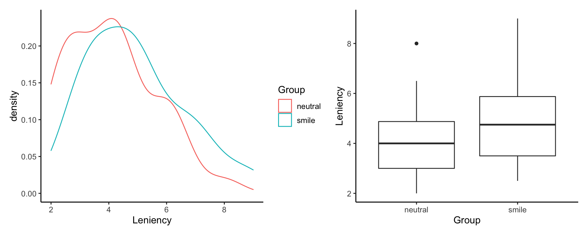
The left panel displays two right skewed distributions. The right panel shows that the median leniency score seems to be higher in the smiling group. There appears to be an outlier in the neutral face expression group, having a leniency score of approximately 8.

Data summary

Let’s now compute the number of participants in each group, as well as the mean leniency score and its standard deviation in each group.

stats <- smiles %>%
  group_by(Group) %>%
  summarise(Count = n(), 
            M = mean(Leniency), 
            SD = sd(Leniency))
stats

# A tibble: 2 x 4
  Group   Count     M    SD
  <chr>   <int> <dbl> <dbl>
1 neutral    34  4.12  1.52
2 smile      34  4.91  1.68

Let’s make the table a pretty HTML table with the gt package. We further format the numeric columns M and SD to be with 2 decimal places only:

library(gt)

gt(stats) %>%
    fmt_number(columns = c(M, SD), decimals = 2)

Group	Count	M	SD
neutral	34	4.12	1.52
smile	34	4.91	1.68

In the sample, the mean leniency score was higher in the smiling group than the neutral expression group. The difference in mean leniency scores between the smiling and neutral group is 0.79.

You can get this by looking at the summary stats:

stats

# A tibble: 2 x 4
  Group   Count     M    SD
  <chr>   <int> <dbl> <dbl>
1 neutral    34  4.12  1.52
2 smile      34  4.91  1.68

The vector corresponding to the column M displays the neutral group first, then the smile group second

stats$M

[1] 4.117647 4.911765

The difference in means between the smiling (2nd group) and neutral group (1st) is:

diff_M <- stats$M[2] - stats$M[1]
diff_M

[1] 0.7941176

Null and alternative hypothesis

The null hypothesis is that facial expression has no effect on the punishment given, i.e. that the population mean leniency score for smiling students is the same as that of neutral students. In other words, there is no difference in population mean leniency score between smiling and neutral students.

The alternative hypothesis, instead, is the claim of interest to the researchers, i.e. that smiling results in a higher mean leniency score compared to non-smiling students.

From the above, we can see that the researchers’ hypothesis that smiling students are given more leniency and milder punishments involves two parameters:

\(\mu_s\) = the population mean leniency score for the smiling students
\(\mu_n\) = the population mean leniency score for students with a neutral expression

We are now ready to formally write the hypotheses being tested:

\[ H_0: \mu_s = \mu_n \\ H_1: \mu_s > \mu_n \]

These can be equivalently written as follows:

\[ H_0: \mu_s - \mu_n = 0 \\ H_1: \mu_s - \mu_n > 0 \]

Note that the statistical hypotheses is about the population difference in means (\(\mu_s - \mu_n\)) and not the sample difference in means, which we know as we have collected data for the sample (difference in means in the sample = 0.79).
Instead, we do not have data for the entire population, and our interest lies in that difference in means for all those in the populations, so for data we don’t have.
This is why we need to perform a formal statistical test to check whether a difference of 0.79 (= the pattern) is large enough compared to the variation in the data due to random sampling (= the noise).

Two-sample t test

To compare the means across 2 groups, we will perform a two-sample t-test. The hypotheses involve two groups, “smile” and “neutral”.

In R this is performed with the t.test() function, but you need to be careful. You need to make the group variable into a factor, and clearly specify the order of the levels. The function t.test() will compute the difference between the mean of the first level - the the mean of the second level.

Factor

Make the column Group into a factor, the levels should be “smile” and “neutral”, and we want smile before neutral, so that t.test will do the mean of smile - mean of neutral.

smiles$Group <- factor(smiles$Group, levels = c('smile', 'neutral'))

Equal variances?

Do the two groups have equal variances? Check this with a variance test var.test():

var.test(Leniency ~ Group, data = smiles)


    F test to compare two variances

data:  Leniency by Group
F = 1.2183, num df = 33, denom df = 33, p-value = 0.5738
alternative hypothesis: true ratio of variances is not equal to 1
95 percent confidence interval:
 0.6084463 2.4393924
sample estimates:
ratio of variances 
          1.218294

Yes, so we will set the var.equal = ... argument of t.test() to TRUE. If the p-value was significant, we would set var.equal = FALSE.

t-test

We finally perform the t-test. In this case, our alternative hypothesis was directional, that the leniency was higher for smiling participants than non-smiling ones. The options for the alternative argument in R are alternative = “two.sided”, “less”, or “greater”. In our case we want “greater”:

smiles_test <- t.test(Leniency ~ Group, data = smiles, var.equal = TRUE,
                      alternative = "greater")
smiles_test


    Two Sample t-test

data:  Leniency by Group
t = 2.0415, df = 66, p-value = 0.0226
alternative hypothesis: true difference in means between group smile and group neutral is greater than 0
95 percent confidence interval:
 0.1451938       Inf
sample estimates:
  mean in group smile mean in group neutral 
             4.911765              4.117647

Understanding the output

The function returns the means of the two groups, which we already computed before in our table of summary statistics.

sample estimates:
  mean in group smile mean in group neutral 
             4.911765              4.117647

stats

# A tibble: 2 x 4
  Group   Count     M    SD
  <chr>   <int> <dbl> <dbl>
1 neutral    34  4.12  1.52
2 smile      34  4.91  1.68

It gives us the t statistics, the degrees of freedom, and the p-value:

t = 2.0415, df = 66, p-value = 0.0226

Recall the t-statistic is the ratio of the pattern to noise, i.e.

\[ t = \frac{\text{pattern}}{\text{noise}} = \frac{\text{observed} - \text{hypothesised difference}}{\text{standard error}} \]

We have the difference in means, computed before and stored into diff_M

diff_M

[1] 0.7941176

The hypothesised difference in means between the smiling and neutral groups is 0, see the null hypothesis.

The standard error is obtained from the t test output:

SE <- smiles_test$stderr
SE

[1] 0.38898

So the t statistic is

(diff_M - 0) / SE

[1] 2.041538

Which matches the output of the t.test function!

t = 2.0415, df = 66, p-value = 0.0226

The degrees of freedom is the sample size, 68, minus the two population means that we don’t know and need to be estimated: 68 - 2 = 66.

The p-value tells us the probability of observing a difference in means more extreme than the one we obtained in the sample, 0.79, if the null hypothesis were true. The p-value is smaller than the significance level of 0.05, meaning that we have strong evidence against the null hypothesis.

Reporting the results

At the 5% significance level, we performed a two-sample t-test against the null hypothesis that the difference in mean leniency score between smiling and non smiling students is equal to zero, with a one-sided alternative that the difference is greater than zero. The test results, \(t(66) = 2.04, p = 0.02\), one-sided, indicate that if smiling truly had no effect on leniency scores, the chance of getting a difference in mean leniency scores between smiling and neutral students as high as 0.79 is 0.02, or 2 in 100 times. The sample data provide strong evidence against the null hypothesis that smiling had no effect on leniency and in favour of the alternative.

General rule

Always report the test results in the context of the study. Link the numbers to the variables under investigation, and provide an interpretation on what the numbers mean in terms of the research question.

The actual t-test results are reported using t(df) = …, p = …

You should always report the p-value in full, perhaps rounded for consistency, unless the p-value is tiny. If it has many decimal places, the reader won’t be interested in the 6th or 7th decimal place. Report any p-value smaller than 0.001 as t(df) = …, p < .001.

Validity conditions of the t-test

In order for the results of the two-sample t-test to be valid, we need that:

The data arise from random assignment of subjects to two groups or from two independent random samples from the population
Either:

Each sample should be sufficiently large (\(n_1 \geq 30, n_2 \geq 30\) as a guideline)

Or:

Both samples came from normal distributions.
Should be described by the study design.
Is checked as follows

smiles %>%
    filter(Group == 'smile') %>%
    pull(Leniency) %>%
    shapiro.test()


    Shapiro-Wilk normality test

data:  .
W = 0.94069, p-value = 0.06464

smiles %>%
    filter(Group == 'neutral') %>%
    pull(Leniency) %>%
    shapiro.test()


    Shapiro-Wilk normality test

data:  .
W = 0.94253, p-value = 0.07335

Both groups appear to be consistent with samples from a normal distribution. The validity conditions are met.

On top of this, also in this case we have the other alternative condition to be true. Both distributions have enough data, 34 in each group, no strong outliers or skeweness:

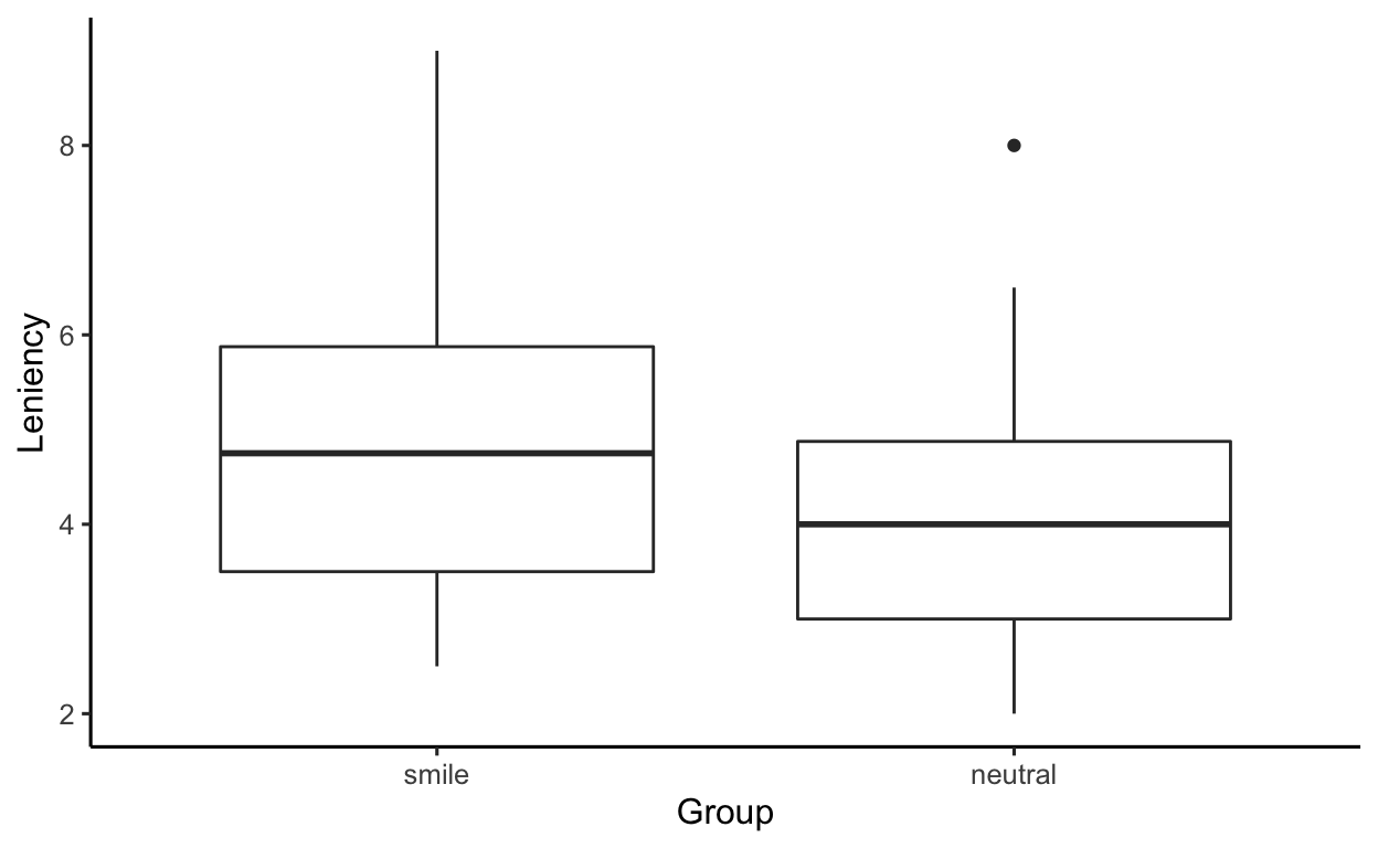
ggplot(smiles, aes(x = Group, y = Leniency)) +
    geom_boxplot()