The “Theory of Planned Behaviour” is a theory about why people engage in certain behaviours. It has been applied in many contexts, and here we are testing the theory as a model of why people exercise.
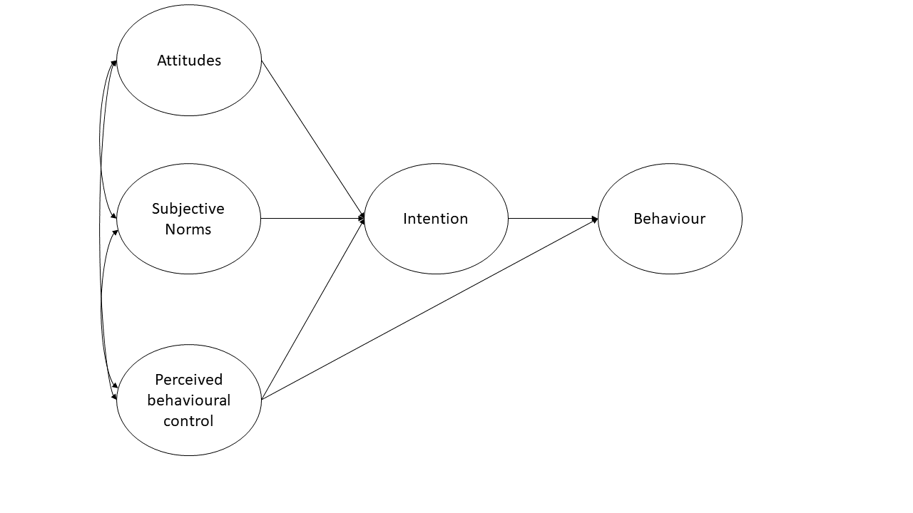
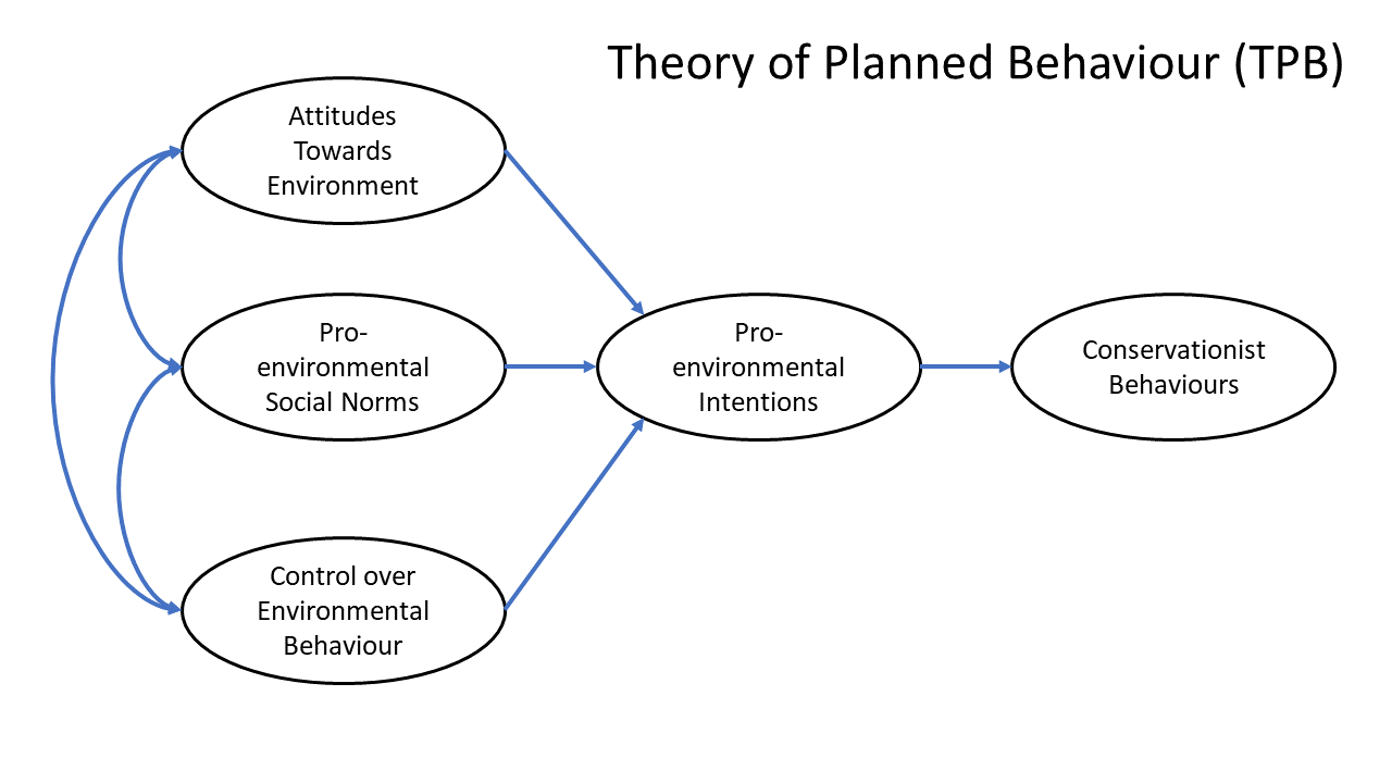
The theory is represented in the diagram in Figure 1 (only the latent variables and not the measured items are shown). Attitudes refer to the extent to which a person has a favourable view of exercising; subjective norms refer to whether they believe others whose opinions they care about believe exercise to be a good thing; and perceived behavioural control refers to the extent to which they believe exercising is under their control. Intentions refer to whether a person intends to exercise and behaviour is a measure of the extent to which they exercised. Each construct is measured using four items apart from intentions which has five.
Figure 1: Theory of planned behaviour (latent variables only)
When I think about people whose opinions matter to me, I believe they value and support regular exercise
SN2
I feel pressure from those I care about to exercise regularly
SN3
Most people who are important to me approve of my exercising
SN4
Most people like me exercise regularly
PBC1
My exercise routine is up to me and only me
PBC2
I am confident that if I want to then I can exercise regularly
PBC3
I believe I have the ability to overcome any obstacles that may prevent me from exercising regularly.
PBC4
I feel capable of sticking to a consistent exercise schedule, even when faced with challenges or distractions
attitude1
I see exercising as an enjoyable and rewarding activity.
attitude2
I believe that exercising contributes positively to my overall well-being and health.
attitude3
I view exercising as an important part of maintaining a healthy lifestyle.
attitude4
I feel energized and invigorated after engaging in physical exercise.
int1
I am determined to take concrete steps towards establishing a consistent exercise habit
int2
I intend to exercise for at least 20 minutes, three times per week for the next three months.
int3
I have made a firm decision to prioritize exercise and allocate time for it in my schedule
int4
I intend to be in shape within the next three months.
int5
I am committed to incorporating regular exercise into my weekly routine.
beh1
I currently engage in physical activity for at least 20 minutes, three times per week, as recommended.
beh2
I already allocate time for exercise in my weekly schedule and adhere to it regularly.
beh3
I track my exercise sessions and ensure I meet my weekly goals
beh4
I do not currently exercise enough
Question 1
Load in the various packages you will probably need (tidyverse, lavaan), and read in the data using the appropriate function.
We’ve given you .csv files for a long time now, but it’s good to be prepared to encounter all sorts of weird filetypes. Can you successfully read in from both types of data?
Our fit is good: RMSEA<.05, SRMR<.05, TLI>0.95 and CFI>.95.
We should also check that all loadings are significant and \(>|.30|\).
To save space I am going to not show the entire summary output here, but just pull out the parameter estimates:
parameterestimates(att_mod.est)
        lhs op       rhs   est    se      z pvalue ci.lower ci.upper
1       att =~ attitude1 0.682 0.051 13.355      0    0.582    0.782
2       att =~ attitude2 0.617 0.045 13.656      0    0.528    0.705
3       att =~ attitude3 0.681 0.049 13.928      0    0.585    0.777
4       att =~ attitude4 0.644 0.048 13.415      0    0.550    0.738
5 attitude1 ~~ attitude1 1.097 0.069 15.883      0    0.961    1.232
6 attitude2 ~~ attitude2 0.837 0.054 15.498      0    0.731    0.943
7 attitude3 ~~ attitude3 0.959 0.063 15.121      0    0.835    1.084
8 attitude4 ~~ attitude4 0.966 0.061 15.809      0    0.847    1.086
9       att ~~       att 1.000 0.000     NA     NA    1.000    1.000
They all look good!
Solution 3. Following the same logic as for the Attitudes, let’s fit the CFA for Subjective norms. Again, all fit measures are very good, and loadings are all significant at greater than 0.3.
Solution 4. All good with Perceived Behavioural Control!
Almost too good (TLI>1, and RMSEA is coming out at exactly 0!), but this is most probably because of this being fake data.
When data is simulated based on a specific model, then fitting that same model structure to the data will obviously fit extremely well! s
It looks like correlating the residuals for items int2 and int4 would improve our model. The expected correlation is 0.757, which is fairly large (remember correlations are between -1 and 1).
Note that the items have a possible theoretical link too, beyond just “intention to exercise”. It looks like both int2 and int4 are specifically about intentions in the next three months. It might make sense that responses to these two items are related more than just representing general ‘intention’.
When we include this covariance, our model fit looks much better!
Solution 6. Finally, the behaviour model looks absolutely fine.
Note that bey4 has a negative loading, which is perfectly okay. In fact, if you look at the items, you’ll notice that this is the only item that is reversed (higher scores on the item reflect less exercising)
Using lavaan syntax, specify the full structural equation model that corresponds to the model in Figure 1. For each construct use the measurement models from the previous question.
Estimate and evaluate the model
Does the model fit well?
Are the hypothesised paths significant?
Hints
This involves specifying the measurement models for all the latent variables, and then also specifying the relationships between those latent variables. All in the same model!
Solution 7.
TPB_model<-' # measurement models att =~ attitude1 + attitude2 + attitude3 + attitude4 SN =~ SN1 + SN2 + SN3 + SN4 PBC =~ PBC1 + PBC2 + PBC3 + PBC4 intent =~ int1 + int2 + int3 + int4 + int5 beh =~ beh1 + beh2 + beh3 + beh4 # covariances between items int2 ~~ int4 # regressions beh ~ intent + PBC intent ~ att + SN + PBC # covariances between attitudes, SN, and PBC att ~~ SN att ~~ PBC SN ~~ PBC'
We can estimate the model using the sem() function.
As with cfa(), by default the sem() function will scale the latent variables by fixing the loading of the first item for each latent variable to 1.
We can see that the model fits well according to RMSEA, SRMR, TLI and CFI.
From the output below, all of the hypothesised paths in the theory of planned behaviour are statistically significant.
Examine the modification indices and expected parameter changes - are there any additional parameters you would consider including?
Solution 8. Making adjustments our theoretical model in order to better represent this sample, we are risking a) over-fitting to the specifics of this sample, and b) testing a theory that we didn’t really have a priori (i.e. we didn’t have this theoretical model before seeing this data).
However, it can still be worth looking at modindices in order to assess any places of local misfit in the model. These can provide useful discussion points and make us pause for thought, even if we are happy with our current model fit.
In this case, none of the expected parameter changes are very large.
Test the indirect effect of attitudes, subjective norms, and perceived behavioural control on behaviour via intentions.
Remember, when you fit the model with sem(), use se='bootstrap' to get boostrapped standard errors (it may take a few minutes). When you inspect the model using summary(), get the 95% confidence intervals for parameters with ci = TRUE.
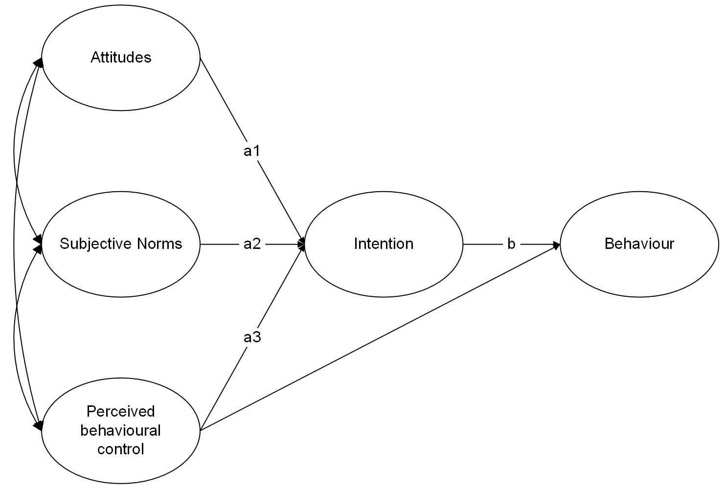
Solution 9. First, let’s name the paths in the structural equation model:
To test these indirect effects we create new a parameter for each indirect effect:
TPB_model2 <-' # measurement models att =~ attitude1 + attitude2 + attitude3 + attitude4 SN =~ SN1 + SN2 + SN3 + SN4 PBC =~ PBC1 + PBC2 + PBC3 + PBC4 intent =~ int1 + int2 + int3 + int4 + int5 beh =~ beh1 + beh2 + beh3 + beh4 # covariances between items int2 ~~ int4 # regressions beh ~ b*intent + PBC intent ~ a1*att + a2*SN + a3*PBC # covariances between attitudes, SN, and PBC att ~~ SN att ~~ PBC SN ~~ PBC # indirect effects: ind1 := a1*b #indirect effect of attitudes via intentions ind2 := a2*b #indirect effect of SN via intentions ind3 := a3*b #indirect effect of PBC via intentions'
When we estimate the model, we request bootstrapped standard errors:
We can see that all of the indirect effects are statistically significant at p<.05 as none of the 95% confidence intervals for the coefficients include zero.
Question 6
Write up your analysis as if you were presenting the work in academic paper, with brief separate ‘Method’ and ‘Results’ sections
Solution 10. Method
We tested a theory of planned behaviour model of physical activity by fitting a structural equation model in which attitudes, subjective norms, perceived behavioural control, intentions and behaviour were latent variables defined by four items. We first tested the measurement models for each construct by fitting a one-factor CFA model. Latent variable scaling was by fixing the loading of the first item for each construct to 1.
Within the SEM, behaviour was regressed on intentions and perceived behavioural control and intentions were regressed on attitudes, subjective norms, and perceived behavioiural control. In addition, attitudes, subjective norms, and perceived behavioural control were allowed to covary. The indirect effects of attitudes, subjective norms and perceived behavioural control on behaviour were calculated as the product of the effect of the relevant predictor on the mediator (intentions) and the effect of the mediator on the outcome. The statistical significance of the indirect effects were evaluated using bootstrapped 95% confidence intervals with 1000 resamples.
In all cases models were fit using maximum likelihood estimation and model fit was judged to be good if CFI and TLI were \(>.95\) and RMSEA and SRMR were \(<.05\). Modification indices and expected parameter changes were inspected to identify any areas of local mis-fit but model modifications were only made if they could be justified on substantive grounds.
Results
All measurement models fit well (CFI and TLI \(>.95\) and RMSEA and SRMR \(<.05\)) with the exception of the measurement model for intentions. Modification indices suggested the inclusion of residual covariance between two items on the intentions scale (int2 and int4) that both made specific reference to short term intentions. The addition of this parameter resulted in a good fit. The full structural equation model (with the residual covariance between int2 and int4 included) fit well (CFI = 0.99, TLI = 0.99, RMSEA = 0.01, SRMR = 0.03). Unstandardised parameter estimates are provided in Table 2. All of the hypothesised paths were statistically significant at \(p<.05\). Significant indirect effects suggested that intentions mediate the effects of attitudes, subjective norms, and perceived behavioural control on behaviour whilst perceived behavioural control also has a direct effect on behaviour. Results thus provide support for a theory of planned behaviour model of physical activity.
Table 2: Unstandardised parameter estimates for structural equation model for a theory of planned behaviour model of physical activity. Note: PBC = Perceived Behavioural Control, CI = Confidence Interval
Parameter
Estimate
SE
z
p
95% CI
Loadings
Attitudes
attitude1
0.69
0.05
14.15
<0.001
[0.59, 0.78]
attitude2
0.61
0.04
13.90
<0.001
[0.53, 0.7]
attitude3
0.66
0.05
14.33
<0.001
[0.57, 0.75]
attitude4
0.66
0.05
14.64
<0.001
[0.57, 0.75]
Subjective Norms
SN1
0.64
0.05
13.95
<0.001
[0.55, 0.73]
SN2
0.59
0.05
12.96
<0.001
[0.5, 0.69]
SN3
0.57
0.04
12.95
<0.001
[0.49, 0.66]
SN4
0.62
0.05
13.00
<0.001
[0.52, 0.72]
PBC
PBC1
0.69
0.04
17.60
<0.001
[0.61, 0.77]
PBC2
0.62
0.04
17.15
<0.001
[0.54, 0.68]
PBC3
0.61
0.04
15.05
<0.001
[0.52, 0.69]
PBC4
0.68
0.04
15.87
<0.001
[0.59, 0.76]
Intentions
int1
0.65
0.04
16.12
<0.001
[0.57, 0.73]
int2
0.55
0.03
16.65
<0.001
[0.49, 0.62]
int3
0.64
0.04
16.87
<0.001
[0.57, 0.72]
int4
0.59
0.04
15.92
<0.001
[0.51, 0.66]
int5
0.53
0.03
17.38
<0.001
[0.47, 0.59]
Behaviours
beh1
0.56
0.04
14.36
<0.001
[0.48, 0.63]
beh2
0.59
0.04
15.13
<0.001
[0.51, 0.66]
beh3
0.64
0.04
16.23
<0.001
[0.56, 0.71]
beh4
-0.60
0.04
-15.18
<0.001
[-0.68, -0.53]
Covariances
int2 with int4
0.31
0.04
8.15
<0.001
[0.23, 0.38]
Attitudes with Subjective Norms
0.32
0.05
6.31
<0.001
[0.22, 0.41]
Attitudes with PBC
0.25
0.05
4.94
<0.001
[0.15, 0.34]
Subjective Norms with PBC
0.27
0.05
5.56
<0.001
[0.18, 0.37]
Regressions
Behaviours on Intentions
0.47
0.06
8.24
<0.001
[0.35, 0.58]
Behaviours on PBC
0.25
0.07
3.79
<0.001
[0.13, 0.38]
Intentions on Attitudes
0.24
0.07
3.67
<0.001
[0.12, 0.37]
Intentions on Subjective Norms
0.33
0.06
5.20
<0.001
[0.21, 0.48]
Intentions on PBC
0.34
0.06
5.48
<0.001
[0.23, 0.47]
Indirect effects
Attitudes via Intentions
0.11
0.03
3.48
<0.001
[0.05, 0.19]
Subjective Norms via Intentions
0.16
0.03
4.47
<0.001
[0.09, 0.23]
PBC via Intentions
0.16
0.03
4.68
<0.001
[0.1, 0.23]
Models of pro-environmental behaviour
Warning: ambiguity incoming!!
In some fields, theories are built on top of immutable laws and well defined measures of physical quantities. In much of the behavioural and social sciences, theories can feel a bit more like a “free-for-all”, working with broad, overlapping concepts that are hard to define, let alone measure. It’s not bad, just very difficult!
This next set of exercises are loosely inspired by Kaiser et al., 2006 :Contrasting the Theory of Planned Behavior With the Value-Belief-Norm Model in Explaining Conservation Behavior, and provide an example of how confusing it is to work in this sort of area.
Dataset: consvmodels.csv
The “theory of planned behaviour” (TPB) is a broad psycho-social theory of ‘why people do things’, that you can find applied in all sorts of contexts, from health psychology to business/organisation psychology, to environmental psychology. Broadly speaking, the theory suggests that we do things because they are beneficial, socially acceptable, and do-able.
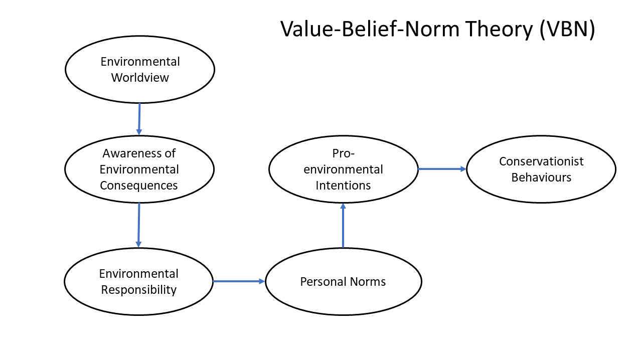
A contrasting theory, specifically for why people take pro-environmental actions, suggests that we do things because our values inform an ‘environmental worldview’ (a set of beliefs about the state of the world), and this in turn results in taking more pro-environmental actions because it encourages us to consider the consequences of our actions and thus our responsibility and our “Personal Norms” (i.e., our personal moral obligation toward the environment). This theory — the “Value-Belief-Norm (VBN) theory” — contrasts with the TPB idea in that it views behavior as a moral response rather than a rational choice. Essentially, the TPB suggests a decision is made by asking ‘is this action good for me and my social standing?’, where the VBN equivalent question would be ‘is this action the right thing to do based on my duty to the planet?’
We’re going to compare these two theories in terms of how well they predict pro-environmental actions.
We have data from 500 people, all of whom filled out a questionnaire that contained 48 items, measuring each of the constructs involved in both TBP and VBN.
Protecting the environment is beneficial and advantageous for society.
att2
Taking action to help the environment feels satisfying and rewarding to me.
att3
I believe acting in an environmentally friendly way is a sensible and effective thing to do.
att4
Environmental conservation is a wise and productive use of my time.
att5
Overall, I have a highly positive and favorable view of being 'green'.
sn1
I feel social pressure to be more environmentally conscious in my daily life.
sn2
People expect each other to protect the environment.
sn3
People whose opinions I value would approve of people making 'green' choices.
sn4
Many people I look up to take active steps to help the environment.
sn5
Most people who are important to me think I should act environmentally friendly.
pbc1
I am confident that I can perform pro-environmental behaviors if I want to.
pbc2
I have the resources and opportunities I need to protect the environment.
pbc3
For me, living an environmentally friendly lifestyle is easy.
pbc4
Whether or not I act environmentally friendly is entirely up to me.
pbc5
I have complete control over how much I contribute to environmental protection.
int1
I intend to take action to protect the environment in the next month.
int2
I plan to reduce my environmental footprint significantly.
int3
I will make a conscious effort to engage in pro-environmental behaviors.
int4
I am determined to choose 'green' alternatives whenever possible.
int5
I expect to increase my level of environmental conservation in the near future.
nep1
The balance of nature is very delicate and easily upset by human activities.
nep2
Humans are severely abusing the environment.
nep3
Plants and animals have as much right as humans to exist.
nep4
The earth is like a spaceship with very limited room and resources.
nep5
Humans must live in harmony with nature in order to survive.
awar1
If we don't act now, the damage to our ecosystem will be irreversible.
awar2
Climate change will have dangerous consequences for my health and safety.
awar3
I believe that environmental problems have a direct impact on my community.
awar4
Environmental protection will help ensure a better life for future generations.
awar5
Environmental pollution is a major threat to all living things on Earth.
resp1
I feel personally responsible for the environmental problems caused by my lifestyle.
resp2
My individual actions can make a meaningful difference in the environment.
resp3
Every person is responsible for the protection of the natural world.
resp4
I believe I have a duty to help solve the environmental issues we face today.
resp5
I feel a sense of ownership over the environmental impact of my household.
pn1
Protecting the environment is a duty I owe to society and/or the planet.
pn2
I would feel guilty and at fault if I did not take action to help the environment.
pn3
I believe acting in an environmentally friendly way is a morally right and necessary thing to do.
pn4
My conscience would bother me if I ignored environmental issues.
pn5
Overall, I feel that being 'green' is a core requirement of my personal values.
cb1
Consumer Choice: I chose to buy products with less packaging or products made from recycled materials.
cb2
Waste Management: I made a conscious effort to sort and recycle my household waste (paper, plastic, glass).
cb3
Resource Conservation: I reduced my water consumption by taking shorter showers or turning off the tap while brushing teeth.
cb4
Sustainable Shopping: I brought my own reusable bags or containers when shopping to avoid using plastic bags.
cb5
Energy Efficiency: I turned off lights and electronic devices in rooms that were not being used to save electricity.
cb6
Transportation: I opted for public transport, cycling, or walking instead of driving a private car for short trips.
cb7
Chemical Reduction: I used eco-friendly cleaning products or avoided using harsh chemicals in my home/garden.
cb8
Temperature Control: I kept the heating/cooling in my home at a lower/higher setting than usual to save energy.
Question 7
Read in the data. It’s all nice and cleaned and ready to go.
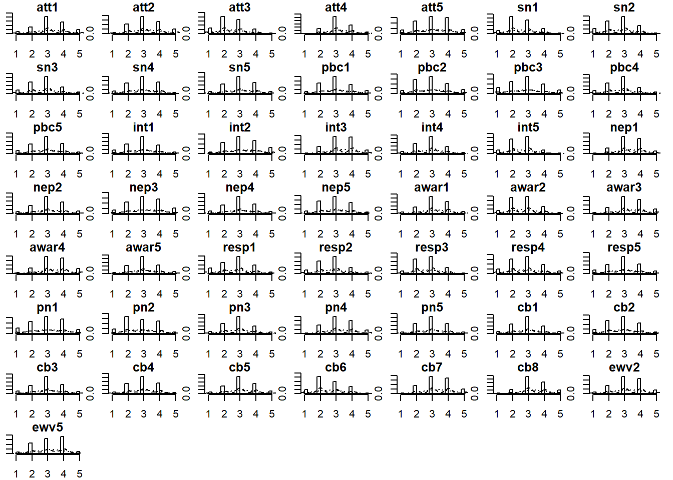
Get some quick plots of item distributions to check things look normal, and get a nice table of descriptive stats for all the variables - stuff like skew and kurtosis.
Hints
the functions (both from the psych package) like multi.hist() and describe() are designed for exactly this purpose - quick explorations of lots and lots of variables.
Here are all the distributions of the variables. They look pretty good — fairly normally distributed (as close as one can get with Likert data) — and we’ve got all 5 responses options being used
library(psych)multi.hist(condat)
And we’re not seeing any problems with skew or kurtosis
In order to compare how well these two theories predict the pro-environmental behaviour, we’re going to want to specify and fit two models, one for the TPB and the other for the VBN theory, but with the same outcome.
Note that in our diagram, that last bit of the two models is the same, going from Intentions->Behaviours.
Before you get started with modelling, check your measurement models for the different constructs, and make any modifications that you deem to be justifiable in order to achieve good fit.
Hints
It’s a pain having to write these all out, so if you want to save time you can copy-paste these:
Solution 12. Here’s the various fit metrics we get, along with the suggested modifications for the three models that don’t fit great.
model
srmr
rmsea
cfi
tli
suggested_adj
Attitudes
0.028
0.000
1.000
1.030
Responsibility
0.019
0.000
1.000
1.077
Environmental Worldview
0.030
0.027
0.994
0.987
Intentions
0.032
0.037
0.988
0.976
Conservationist Behaviours
0.043
0.044
0.978
0.969
Social Norms
0.048
0.060
0.935
0.869
sn1~~sn5
Planned Behavioural Control
0.035
0.064
0.976
0.953
pbc4~~pbc5
Personal Norms (Environmental Conscientiousness)
0.052
0.109
0.926
0.853
pn2~~pn4
Awareness of Consequences
0.062
0.124
0.885
0.769
awar1~~awar4
All important - we shouldn’t just shove these adjustments in without considering if they make theoretical sense.
# A tibble: 8 × 2
  variable wording
  <chr>    <chr>
1 sn1      I feel social pressure to be more environmentally conscious in my da…
2 sn5      Most people who are important to me think I should act environmental…
3 pbc4     Whether or not I act environmentally friendly is entirely up to me.
4 pbc5     I have complete control over how much I contribute to environmental …
5 awar1    If we don't act now, the damage to our ecosystem will be irreversibl…
6 awar4    Environmental protection will help ensure a better life for future g…
7 pn2      I would feel guilty and at fault if I did not take action to help th…
8 pn4      My conscience would bother me if I ignored environmental issues.
The question we are asking ourselves here is if there is reason that these pairs of variables might be related beyond their relations to the overall constructs.
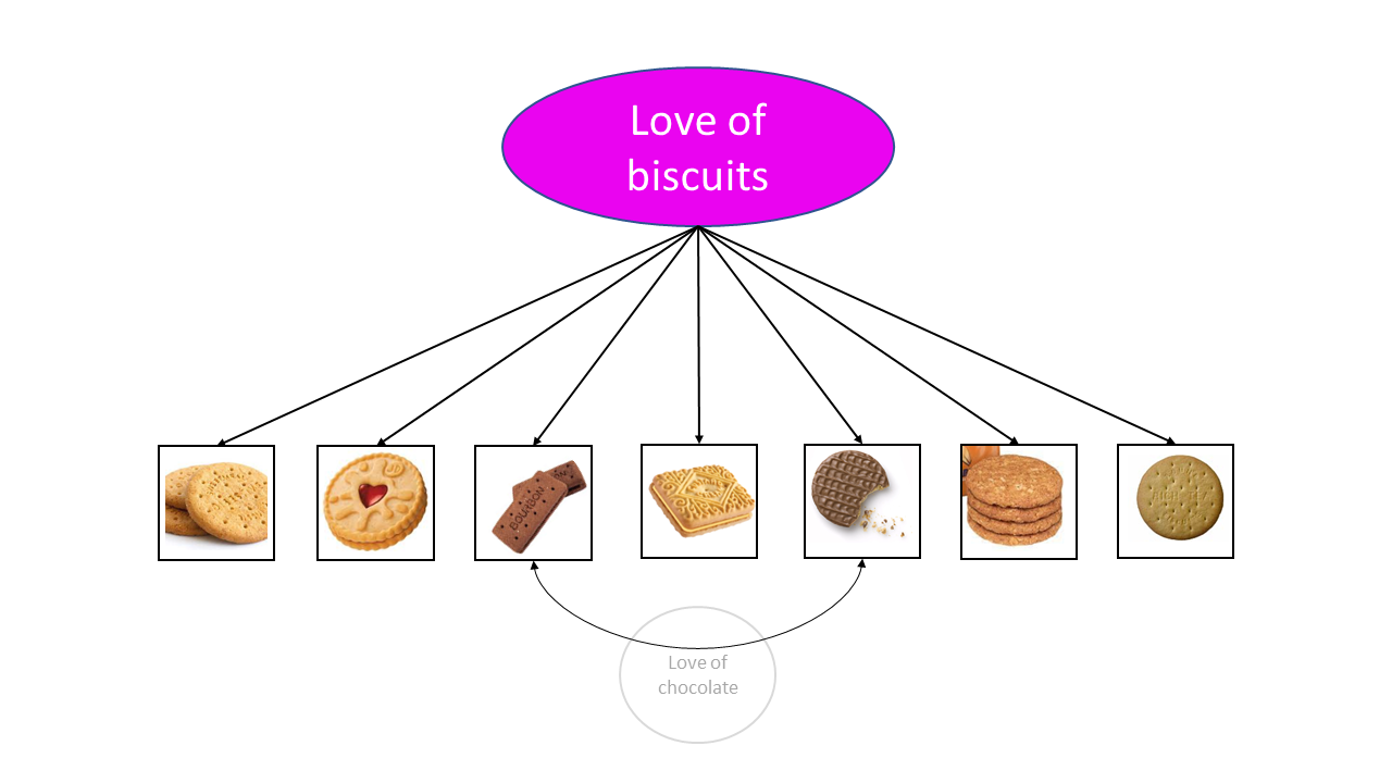
My go-to example for this idea is to imagine a measurement of “love of biscuits” where we rate how much we like lots different types of biscuits. If our scale contains ratings for 7 biscuits, 2 of which are chocolate flavoured, then we can justifiably see a reason why those two ratings will be related beyond their representation of ‘love of biscuits’ - they will be more related because they specifically represent ‘love of chocolate’!
A residual correlation here is kind of just like a suggestion of some other latent factor. We don’t need to explicitly model it, because this factor would be underidentified (a factor needs 3 indicators remember):
In this example, I can sort of see that while pn2 and pn4 both capture “Personal Norms” - they both capture personal expectations of behaviours - but they are both specifically about feelings of guilt.
Similarly, pbc1 and pbc5 are specifically about complete freedom/control over environmental actions.
It’s slightly harder to see the link between awar1 and awar4 - they’re both possibly a bit more ‘long-term’-focused than the other awar- items? The sn1 and sn5 link could be that they are both specifically about perceived pressure from friends and family, rather than social norms in general.
(I find this part makes me feel a little ¯\(ツ)/¯ - it feels like I could probably persuade myself of a link between almost any pair of sentences!)
Here are the fit measures after we make these modifications:
model
srmr
rmsea
cfi
tli
Social Norms - adj
0.030
0.000
1.000
1.006
Awareness of Consequences - adj
0.033
0.053
0.983
0.958
Personal Norms - adj
0.033
0.071
0.975
0.938
Planned Behavioural Control - adj
0.034
0.075
0.974
0.936
Question 9
Okay, let’s now move to specifying and fitting models that reflect our two theories - TPB and VBN. Do they fit well? are all of the hypothesised paths are significant?
They do fit okay.. ish.. Let’s be a bit more lenient here - these thresholds are just arbitrary, after all!)
If we take a look at the summary() of each, we’ll see that all the relevant paths are significant.
Question 10
Our question is about how well these two theories predict conservationist behaviours.
We’re using the same outcome - conservationist behaviours - so what we would like to know is how much variance in the outcome is explained in each of our models.
We can do that!
inspect(model, what ="rsquare")
Which theory explains more variability in how people engage in pro-environmental behaviours?
Solution 14.
inspect(tpb.est, what ="rsquare")['Conserv_Beh']
Conserv_Beh
  0.5533943
inspect(vbn.est, what ="rsquare")['Conserv_Beh']
Conserv_Beh
  0.5494775
TPB explains more, but only just… only ~0.39% more variability in behaviours is explained by TPB compared to VBN
Solution 15. Because both models have Intentions as the direct proximal (nearest) cause of Conservationist Behaviours, of course they’re going to explain similar amounts..
What may be a better thing to look at is how well we are predicting Intentions?
Here we see a slightly different picture - in explaining intentions, the TPB is doing a much better job - explaining almost 5 times as much variability in how much people intend to act in pro-environmental ways.
inspect(tpb.est, what ="rsquare")['Intentions']
Intentions
 0.4938615
inspect(vbn.est, what ="rsquare")['Intentions']
Intentions
 0.1124297
Question 11
Let’s take stock of where we are now. We’ve got two competing theories about why people act in environmentally friendly ways. Both theories provide overall good fit to the data. They explain a similar amount of variance in our final outcome measure of conservationist behaviours, but the TPB provides a better prediction of peoples intentions.
To do some more thorough work, we might want to think a bit more about how exactly these two theories differ. If we take a step back a bit, both of these theories are just saying “Something–>Intentions–>Actions”, and they differ in terms of what they say explains why people have different intentions. TPB says our intentions are driven by 3 things (Attitudes, Social Pressure, and amount of control we think we have over our actions), and VBN says they are driven by a chain of things that results in a Personal sense of moral obligation (“Personal Norms”).
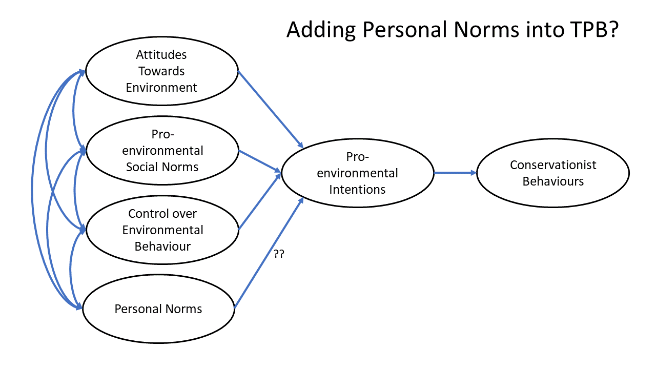
So one way we could start to think about assessing these theories, is to ask if the addition of the “Personal Norms” part of VBN provides explanatory power beyond the other parts of the TPB, i.e.:
Fit the model presented in the diagram above. What do you conclude (if anything?)
Solution 16. All we need to do is add in the Personal Norms to our TPB model:
However, the most interesting part for me here is the estimated paths of the model. Let’s look at the paths between the latent variables:
# this just gets the std estimates, and filters to any regressions and covariancesstandardizedsolution(tpb.est2) |>filter(op %in%c("~","~~"), lhs!=rhs)
Note that the paths from both Attitudes and PNorms to Intentions are not significant, and — interestingly — Attitudes and PNorms have a correlation of 0.8!
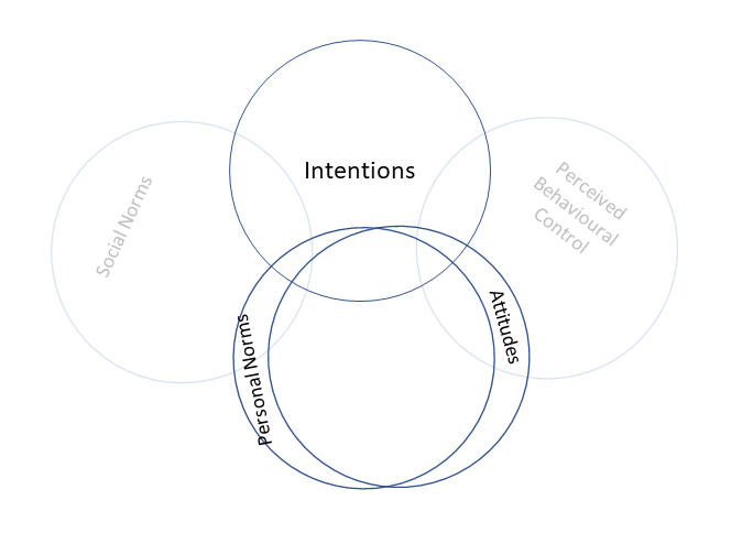
So what’s going on? One likely possibility is that there’s a lot of overlap between all these constructs we’re talking about. For all intents and purposes, the problem here is that “Attitudes” and “Personal Norms” look like pretty much the same thing!
So really, this is all coming down to unclear measurement! If we think about just the Intentions ~ Attitudes + PNorms bit of our model, we’re kind of in this situation, where the overlap is so great that we’re unable to see the unique contributions of either one.
And examination of the item wordings themselves shows how we might have been able to spot this problem beforehand. It’s likely that people aren’t really discerning between the subtleties of these questions.
Attitudes
variable
wording
att1
Protecting the environment is beneficial and advantageous for society.
att2
Taking action to help the environment feels satisfying and rewarding to me.
att3
I believe acting in an environmentally friendly way is a sensible and effective thing to do.
att4
Environmental conservation is a wise and productive use of my time.
att5
Overall, I have a highly positive and favorable view of being 'green'.
Personal Norms
variable
wording
pn1
Protecting the environment is a duty I owe to society and/or the planet.
pn2
I would feel guilty and at fault if I did not take action to help the environment.
pn3
I believe acting in an environmentally friendly way is a morally right and necessary thing to do.
pn4
My conscience would bother me if I ignored environmental issues.
pn5
Overall, I feel that being 'green' is a core requirement of my personal values.
So what’s the take-home from all this? In some respects, it’s that measurement underpins everything we do, and it’s especially pertinent when our theories and research questions are devised at a high level of ambiguous concepts.
So what can we do? Well, the short answer here is “not much”. But that’s because we’re a little too late. We should ideally be thinking about this stuff all prior to collecting data. If we can identify these issues early then we can better define and so measure the constructs involved in our theories.
 In this example, I can sort of see that while