Week 7 Exercises: PCA & EFA

New packages

We’re going to be needing some different packages this week (no more lme4!).
Make sure you have these packages installed:

• psych
  
• GPArotation
  
• car

Reducing the dimensionality of job performance

Data: jobperfbonus.csv

A company has asked line managers to fill out a questionnaire that asks them to capture ‘performance indicators’ for each of their employees. These 15 indicators are a mix of metrics from the companies work management software, and questions about manager’s perceptions of their employees’ work over the last year.

The company’s leadership team finds the 15-indicator report a bit confusing and overwhelming. They want to create a simplified “Performance Dashboard” that captures only the most important directions of variance in their employees.

It can be downloaded at https://uoepsy.github.io/data/jobperfbonus.csv

Table 1: data dictionary for jobperfbonus.csv

variable	question
name	employee name
q1	Deadline Consistency: Average discrepancy between 'Target Date' vs. 'Actual Completion Date' for assigned tasks.
q2	Scheduling: Frequency of updated timelines or revised milestones sent to the team.
q3	Resource Allocation: How well have they allocated resources to ensure efficient project execution?
q4	Risk Identification: Rate their proficiency in identifying and mitigating project risks.
q5	Project Updating: Frequency of weekly status emails/announcements on the project.
q6	Collaboration: Number of projects where they were a 'Collaborator' or 'Contributor' alongside others.
q7	Teamwork: Rate how well they have actively listened to and considered the ideas and opinions of others.
q8	Positivity: How effectively have they contributed to a positive team environment?
q9	Assistance: Frequency of being tagged for help on others' assigned tasks.
q10	Conflict: How well have they resolved conflicts and disagreements within the team?
q11	Technical Proficiency: The number of tasks sent back for 'Correction' versus those approved on the first pass.
q12	Technical Development: Number of completed internal or external training certifications.
q13	Problem Resolution: The average time between a 'Help Ticket' or 'Bug' being assigned and closed.
q14	Technical Communication: How well have they translated complex technical information into understandable terms for non-technical stakeholders?
q15	Technical Initiative: How well have they leveraged technical expertise for problem-solving?

Question 1

Load the data!

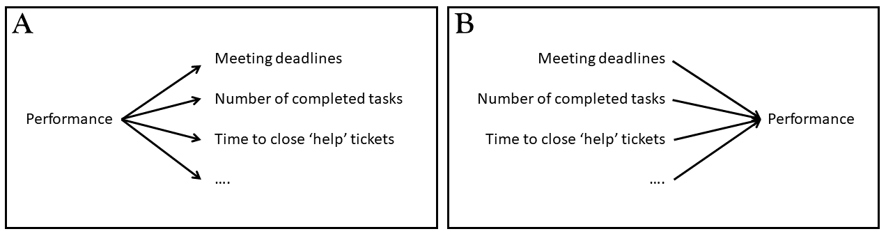
We’re going to want to reduce these 15 variables (or “items”) down into a smaller set. Should we use PCA or EFA?

Solution 1.

jobperf <- read_csv("https://uoepsy.github.io/data/jobperfbonus.csv")
head(jobperf)

# A tibble: 6 × 16
  name      q1    q2    q3    q4    q5    q6    q7    q8    q9   q10   q11   q12
  <chr>  <dbl> <dbl> <dbl> <dbl> <dbl> <dbl> <dbl> <dbl> <dbl> <dbl> <dbl> <dbl>
1 Kang,…   -32   0.6     2     1   0.3    14     2     3  0.06     2  0.6      7
2 Zouni…     4   1.6     3     4   1      20     3     4  0.1      4  0.52     9
3 el-Sy…     0   1.3     3     4   0.7    19     3     4  0.07     3  0.54     3
4 Thomp…   -18   1.2     1     3   0.4    16     2     4  0.09     2  0.81     7
5 Wahl,…     2   1.7     2     3   0.7    14     3     4  0.06     3  0.58     9
6 al-Ko…   -24   0.8     1     1   0      27     3     4  0.08     3  0.59     5
# ℹ 3 more variables: q13 <dbl>, q14 <dbl>, q15 <dbl>

We’re probably going to want to use PCA, because it is hard to understand what an underlying latent dimension of ‘performance’ would be — i.e., it makes more sense to think of any overall measure of ‘performance’ as just being the combination of all of those indicators.

One way to reason about this is to task which of these makes more sense:

• A. If my ‘job performance’ increases, then my scores on the indicators will go up
  
• B. If my scores on the indicators go up, then my ‘job performance’ will increase

Really, we are just asking about the direction of the arrows. Which picture makes more sense?

Question 2

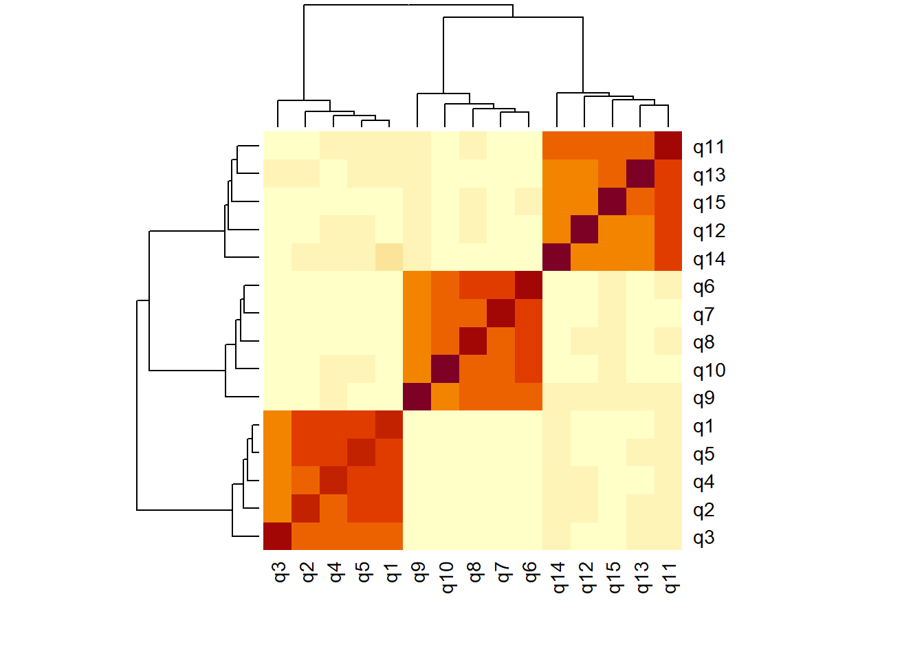
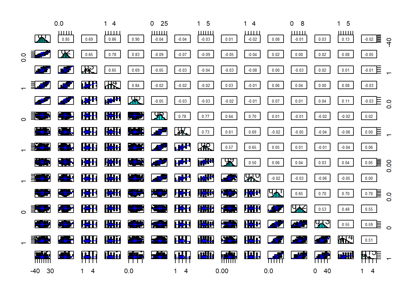
Explore the relationships between variables in the data.

You’re probably going to want to subset out just the relevant variables (q1 to q15).

Hints

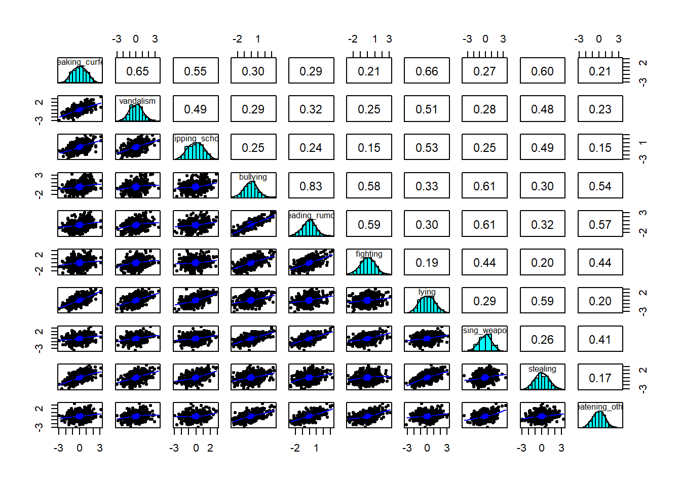
There are lots of variables! There are various things we can do here. Try some of them to see what they do:

• cor(data)
• heatmap(cor(data))
• pairs.panels(data) (from the psych package)

Solution 2. Let’s keep the full data with the names, but make a new object that is just the performance data:

qperf <- jobperf |> select(-name)

It looks like we’ve got some very strong groups of questions there - q1 to q5 are all highly related to one another, as are q6 to q10, and q11 to q15. Furthermore, the relations between those sets are very weak, suggesting 3 groups that are fairly distinct.

heatmap(cor(qperf))

You’ll probably have to zoom in when you do this yourself, as there are a lot of little plots there!

library(psych)
pairs.panels(qperf)

Question 3

How much variance in the set of performance indicators will be captured by 15 principal components?

Note: We can figure this out without having to do anything - it’s a theoretical question!

Solution 3. All of it!
The right hand entry of the “Cumulative Var” row is 1 - it explains everything.

principal(qperf, nfactors = 15, rotate = "none")

Principal Components Analysis
Call: principal(r = qperf, nfactors = 15, rotate = "none")
Standardized loadings (pattern matrix) based upon correlation matrix
      PC1  PC2   PC3   PC4   PC5   PC6   PC7   PC8   PC9  PC10  PC11  PC12
q1   0.90 0.29 -0.15 -0.08 -0.04 -0.02 -0.03 -0.07 -0.06 -0.02  0.00 -0.01
q2   0.87 0.22 -0.17 -0.03 -0.05 -0.06  0.04 -0.13  0.01  0.06  0.29 -0.06
q3   0.75 0.20 -0.17  0.28  0.15  0.28  0.01  0.35  0.23 -0.07 -0.02  0.00
q4   0.85 0.29 -0.16 -0.03  0.02 -0.13 -0.05 -0.07 -0.08  0.02 -0.24  0.13
q5   0.89 0.28 -0.15 -0.03 -0.06 -0.04  0.02 -0.05 -0.06  0.00 -0.02 -0.06
q6  -0.33 0.85 -0.08  0.02 -0.02  0.01  0.02  0.09 -0.10  0.06  0.06  0.35
q7  -0.32 0.83 -0.11  0.03 -0.05  0.08  0.04  0.05  0.02  0.39 -0.06 -0.17
q8  -0.31 0.82 -0.05  0.13 -0.07  0.03 -0.01  0.13 -0.32 -0.23  0.08 -0.14
q9  -0.24 0.73 -0.01 -0.26  0.54  0.03 -0.07 -0.15  0.11 -0.09  0.01 -0.04
q10 -0.29 0.77 -0.11  0.03 -0.35 -0.14  0.04 -0.14  0.35 -0.16 -0.05 -0.01
q11  0.17 0.17  0.89 -0.04 -0.04  0.01 -0.03  0.01 -0.09 -0.05 -0.22 -0.10
q12  0.11 0.10  0.76  0.22  0.18 -0.52  0.11  0.14  0.05  0.04  0.06  0.00
q13  0.15 0.10  0.80  0.05  0.01  0.29  0.44 -0.19 -0.01 -0.02  0.02  0.05
q14  0.22 0.11  0.75 -0.50 -0.16  0.05 -0.09  0.26  0.07  0.01  0.08  0.02
q15  0.07 0.13  0.80  0.28 -0.03  0.16 -0.42 -0.20  0.03  0.05  0.08  0.04
     PC13  PC14  PC15 h2       u2 com
q1  -0.01 -0.11 -0.24  1  1.3e-15 1.5
q2  -0.15  0.16  0.04  1  2.3e-15 1.7
q3  -0.02  0.02  0.00  1  6.7e-16 2.8
q4   0.15  0.19  0.04  1  2.8e-15 1.9
q5   0.03 -0.25  0.16  1  2.6e-15 1.6
q6  -0.13 -0.05  0.01  1  2.2e-16 1.8
q7   0.04  0.01 -0.02  1  5.6e-16 2.0
q8   0.10  0.05  0.00  1  1.1e-16 2.1
q9   0.00 -0.01  0.01  1  1.1e-16 2.6
q10  0.01  0.01  0.00  1  6.7e-16 2.6
q11 -0.29  0.03  0.01  1 -2.0e-15 1.6
q12  0.05 -0.03 -0.02  1 -1.3e-15 2.4
q13  0.09  0.01 -0.01  1 -8.9e-16 2.2
q14  0.11  0.01  0.01  1 -1.8e-15 2.6
q15  0.07 -0.02  0.00  1 -1.6e-15 2.2

                       PC1  PC2  PC3  PC4  PC5  PC6  PC7  PC8  PC9 PC10 PC11
SS loadings           4.20 3.61 3.38 0.55 0.52 0.51 0.41 0.38 0.33 0.26 0.22
Proportion Var        0.28 0.24 0.23 0.04 0.03 0.03 0.03 0.03 0.02 0.02 0.01
Cumulative Var        0.28 0.52 0.75 0.78 0.82 0.85 0.88 0.90 0.93 0.94 0.96
Proportion Explained  0.28 0.24 0.23 0.04 0.03 0.03 0.03 0.03 0.02 0.02 0.01
Cumulative Proportion 0.28 0.52 0.75 0.78 0.82 0.85 0.88 0.90 0.93 0.94 0.96
                      PC12 PC13 PC14 PC15
SS loadings           0.21 0.19 0.14 0.09
Proportion Var        0.01 0.01 0.01 0.01
Cumulative Var        0.97 0.98 0.99 1.00
Proportion Explained  0.01 0.01 0.01 0.01
Cumulative Proportion 0.97 0.98 0.99 1.00

Mean item complexity =  2.1
Test of the hypothesis that 15 components are sufficient.

The root mean square of the residuals (RMSR) is  0 
 with the empirical chi square  0  with prob <  NA 

Fit based upon off diagonal values = 1

Question 4

Remember, the company is wanting us to simplify things down from having 15 indicators of ‘job performance’ to a smaller set, that captures the most important ways in which employees vary in their performance.

We’re going to use PCA.
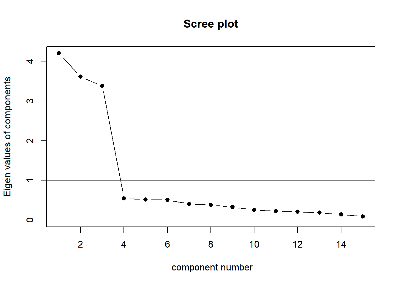
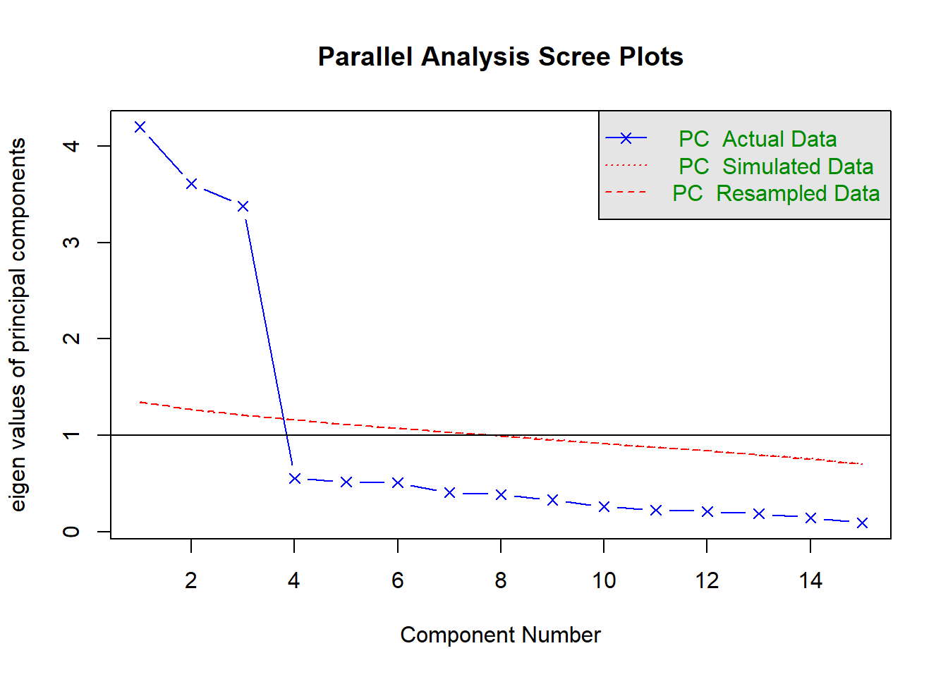
How many components should we keep?

Hints

See scree plots, parallel analysis, MAP - Chapter 2 - PCA walkthrough.

Solution 4. According to Kaiser’s rule, we should keep 3 components

principal(qperf, nfactors = 15, rotate = "none")$values

 [1] 4.20133825 3.61121794 3.37806982 0.55089392 0.51766122 0.50970760
 [7] 0.40518560 0.38424599 0.33003793 0.25868856 0.22449635 0.20892955
[13] 0.18571607 0.14318987 0.09062133

Solution 5. According to the Scree plot, I would suggest keeping 3 components

scree(qperf, factors = FALSE)

Solution 6. According to the MAP, we should keep 3 components

VSS(qperf, n = ncol(qperf), 
    rotate = "none", fm = "pc", plot = FALSE)

Very Simple Structure
Call: vss(x = x, n = n, rotate = rotate, diagonal = diagonal, fm = fm, 
    n.obs = n.obs, plot = plot, title = title, use = use, cor = cor)
VSS complexity 1 achieves a maximimum of 0.96  with  3  factors
VSS complexity 2 achieves a maximimum of 0.98  with  6  factors

The Velicer MAP achieves a minimum of 0.02  with  3  factors 

BIC achieves a minimum of  Inf  with    factors

Sample Size adjusted BIC achieves a minimum of  Inf  with    factors

Statistics by number of factors 
   vss1 vss2   map dof chisq prob sqresid  fit RMSEA BIC SABIC complex eChisq
1  0.41 0.00 0.143   0    NA   NA 2.6e+01 0.41    NA  NA    NA      NA     NA
2  0.70 0.70 0.071   0    NA   NA 1.3e+01 0.70    NA  NA    NA      NA     NA
3  0.96 0.97 0.021   0    NA   NA 1.5e+00 0.97    NA  NA    NA      NA     NA
4  0.96 0.97 0.031   0    NA   NA 1.2e+00 0.97    NA  NA    NA      NA     NA
5  0.84 0.97 0.047   0    NA   NA 9.0e-01 0.98    NA  NA    NA      NA     NA
6  0.84 0.98 0.069   0    NA   NA 6.4e-01 0.99    NA  NA    NA      NA     NA
7  0.76 0.96 0.106   0    NA   NA 4.8e-01 0.99    NA  NA    NA      NA     NA
8  0.75 0.91 0.125   0    NA   NA 3.3e-01 0.99    NA  NA    NA      NA     NA
9  0.67 0.92 0.174   0    NA   NA 2.2e-01 0.99    NA  NA    NA      NA     NA
10 0.67 0.91 0.211   0    NA   NA 1.6e-01 1.00    NA  NA    NA      NA     NA
11 0.67 0.90 0.264   0    NA   NA 1.1e-01 1.00    NA  NA    NA      NA     NA
12 0.61 0.90 0.406   0    NA   NA 6.3e-02 1.00    NA  NA    NA      NA     NA
13 0.59 0.87 0.580   0    NA   NA 2.9e-02 1.00    NA  NA    NA      NA     NA
14 0.59 0.87 1.000   0    NA   NA 8.2e-03 1.00    NA  NA    NA      NA     NA
15 0.59 0.87    NA   0    NA   NA 1.5e-27 1.00    NA  NA    NA      NA     NA
   SRMR eCRMS eBIC
1    NA    NA   NA
2    NA    NA   NA
3    NA    NA   NA
4    NA    NA   NA
5    NA    NA   NA
6    NA    NA   NA
7    NA    NA   NA
8    NA    NA   NA
9    NA    NA   NA
10   NA    NA   NA
11   NA    NA   NA
12   NA    NA   NA
13   NA    NA   NA
14   NA    NA   NA
15   NA    NA   NA

Solution 7. According to the parallel analysis, we should keep 3 components

fa.parallel(qperf, fa="pc", n.iter = 500)

Parallel analysis suggests that the number of factors =  NA  and the number of components =  3 

Solution 8. In this case, everything agrees that we should retain 3 components:

guides	suggestion
Kaiser	3
Scree	3
MAP	3
Parallel Analysis	3

Question 5

Conduct a principal components analysis extracting the number of components you decided on from the previous question.

Be sure to set rotate = "none" (a conventional PCA does not use rotations - it is simply about data reduction. The line is a bit blurred here, but once we start introducing rotations, we are moving more towards a form of EFA).

Examine the loadings for the components. By thinking in relation to the questions that were asked (refer back to Table 1), what do you think each component is capturing?

Solution 9. It’s rarely as neat as this, but we can see the patterns of higher loadings for the groups of 5 questions on each component.

• PC1 has higher loadings for q1 to q5
• PC2 has higher loadings for q6 to q10
• PC3 has higher loadings for q11 to q15

Looking back at the questions in Table 1, questions 1 to 5 were all about stuff related to ‘project management’. Questions 6 to 10 were all about collaboration with team members, and questions 11 to 15 were all about technical skill.

principal(qperf, nfactors = 3, rotate = "none")

Principal Components Analysis
Call: principal(r = qperf, nfactors = 3, rotate = "none")
Standardized loadings (pattern matrix) based upon correlation matrix
      PC1  PC2   PC3   h2    u2 com
q1   0.90 0.29 -0.15 0.91 0.089 1.3
q2   0.87 0.22 -0.17 0.83 0.169 1.2
q3   0.75 0.20 -0.17 0.64 0.361 1.3
q4   0.85 0.29 -0.16 0.83 0.167 1.3
q5   0.89 0.28 -0.15 0.89 0.106 1.3
q6  -0.33 0.85 -0.08 0.83 0.167 1.3
q7  -0.32 0.83 -0.11 0.80 0.200 1.3
q8  -0.31 0.82 -0.05 0.77 0.233 1.3
q9  -0.24 0.73 -0.01 0.59 0.411 1.2
q10 -0.29 0.77 -0.11 0.69 0.315 1.3
q11  0.17 0.17  0.89 0.84 0.155 1.1
q12  0.11 0.10  0.76 0.60 0.398 1.1
q13  0.15 0.10  0.80 0.67 0.327 1.1
q14  0.22 0.11  0.75 0.62 0.378 1.2
q15  0.07 0.13  0.80 0.67 0.334 1.1

                       PC1  PC2  PC3
SS loadings           4.20 3.61 3.38
Proportion Var        0.28 0.24 0.23
Cumulative Var        0.28 0.52 0.75
Proportion Explained  0.38 0.32 0.30
Cumulative Proportion 0.38 0.70 1.00

Mean item complexity =  1.2
Test of the hypothesis that 3 components are sufficient.

The root mean square of the residuals (RMSR) is  0.04 
 with the empirical chi square  134.75  with prob <  3.9e-07 

Fit based upon off diagonal values = 0.99

Question 6

Extract the scores on the principal components.
The company wants to reward teamwork. Pick 10 people they should give a bonus to.

Hints

See Chapter 2#PCA-walkthrough - scores for how to extract scores (a score on each component for each row of our original dataset) using the $scores from the object fitted with principal().

This will contain as many sets of scores as there are components. One of these (given the previous question) might be of use here.

You’ll likely want to join them back to the column of names. So we can figure out who gets the bonus. cbind() or bind_cols() might help here.

Solution 10. The second component seems to capture a lot of ‘teamwork’ related questions. So if we extract scores on that second component, we could then pick the 10 people for whom they are highest on that component.

This will extract the scores:

principal(qperf, nfactors = 3, rotate = "none")$scores

Let’s combine them with the original data that contains the employee names, so we can figure out who to give bonuses to.
We could do this with cbind(), or bind_cols(),

# first we bind the columns of the scores, back to 
# the original data which contains the names
jobperf <- 
  bind_cols(
    principal(qperf, nfactors = 3, rotate = "none")$scores,
    jobperf
  ) 

# we can then choose just the 10 people 
# who have the highest scores on PC2 (the teamwork component)
jobperf |> select(name, PC2) |>
  arrange(desc(PC2))

# A tibble: 400 × 2
   name                 PC2
   <chr>              <dbl>
 1 Robinson, Shayla    2.88
 2 Hunt, Maliek        2.63
 3 Kearns, Sarah       2.40
 4 Billings, Justin    2.39
 5 Phillips, Nashelle  2.33
 6 al-Masih, Sawada    2.26
 7 Vargas, Joseph      2.16
 8 Reider, Samuel      2.12
 9 Dhanoa, Eunice      2.10
10 Brown, Jameela      1.98
# ℹ 390 more rows

Understanding Conduct Problems

Data: Conduct Problems

A researcher is developing a new brief measure of Conduct Problems. She has collected data from n=450 adolescents on 10 items, which cover the following behaviours:

1. Breaking curfew
2. Vandalism
3. Skipping school
4. Bullying
5. Spreading malicious rumours
6. Fighting
7. Lying
8. Using a weapon
9. Stealing
10. Threatening others

Our task is to use the dimension reduction techniques we learned about in the lecture to help inform how to organise the items she has developed into subscales.

The data can be found at https://uoepsy.github.io/data/conduct_probs_scale.csv

Question 7

Read in the dataset.
Create a correlation matrix for the items, and inspect the items to check their suitability for exploratory factor analysis (see Chapter 3#EFA-initial checks).

Solution 11.

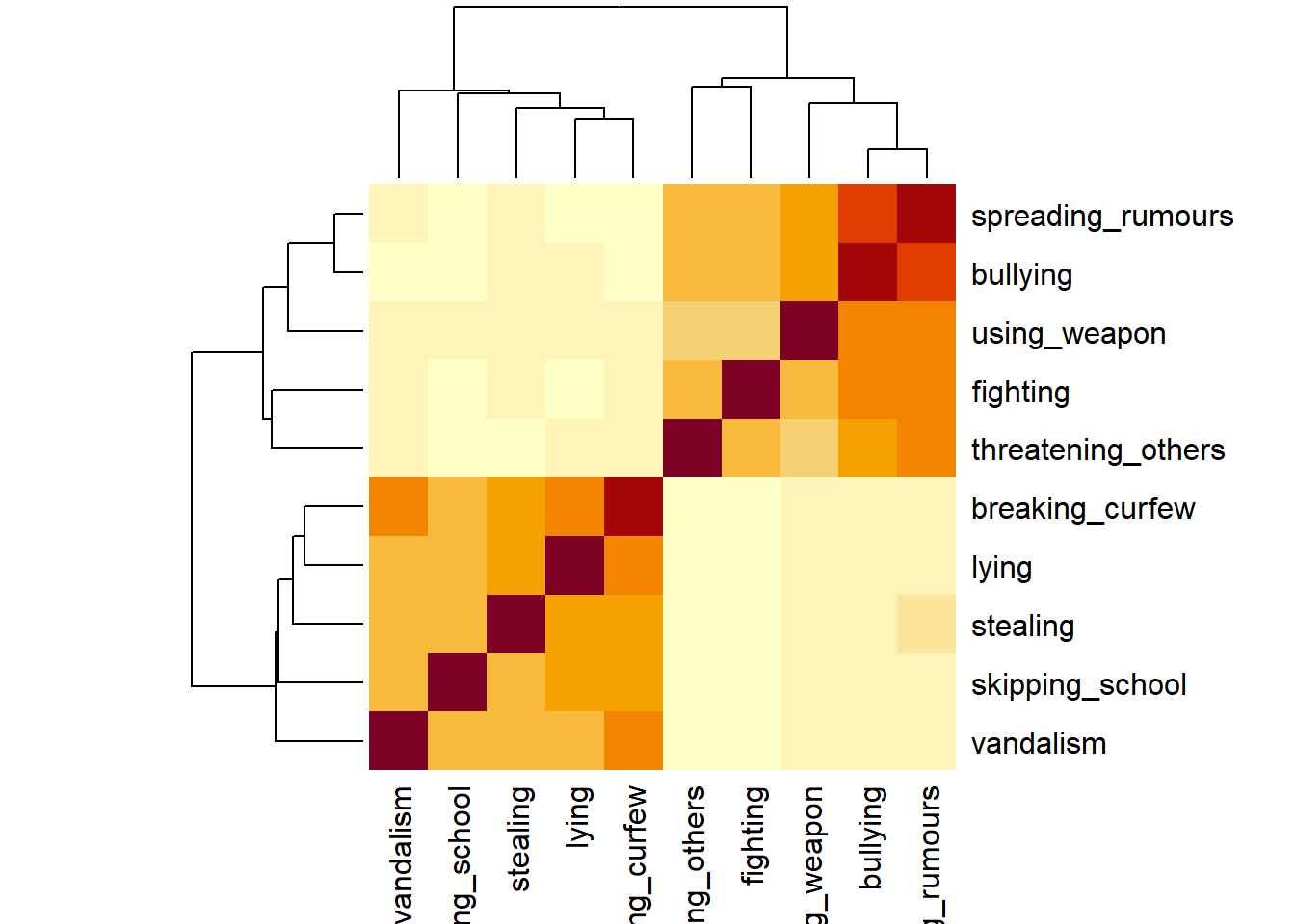
cpdata <- read.csv("https://uoepsy.github.io/data/conduct_probs_scale.csv")
# discard the first column
cpdata <- cpdata[,-1]

Here’s a correlation matrix. There’s no obvious blocks of items here, but we can see that there are some fairly high correlations, as well as some weaker ones. All are positive.

heatmap(cor(cpdata))

The Bartlett’s test comes out with a p-value of 0 (which isn’t possible, but it’s been rounded for some reason). This suggests that we reject the null of this test (that our correlation matrix is proportional to the identity matrix). This is good. It basically means “we have some non-zero correlations”!

cortest.bartlett(cor(cpdata), n=450)

$chisq
[1] 2237.533

$p.value
[1] 0

$df
[1] 45

The overall sampling adequacy is 0.87, which is pretty good! (or rather, which is ‘meritorious’!). MSA for all items is >.8

KMO(cpdata)  

Kaiser-Meyer-Olkin factor adequacy
Call: KMO(r = cpdata)
Overall MSA =  0.87
MSA for each item = 
   breaking_curfew          vandalism    skipping_school           bullying 
              0.84               0.88               0.92               0.82 
 spreading_rumours           fighting              lying       using_weapon 
              0.81               0.94               0.88               0.95 
          stealing threatening_others 
              0.90               0.94 

Finally, all the relationships here look fairly linear:

pairs.panels(cpdata)

Question 8

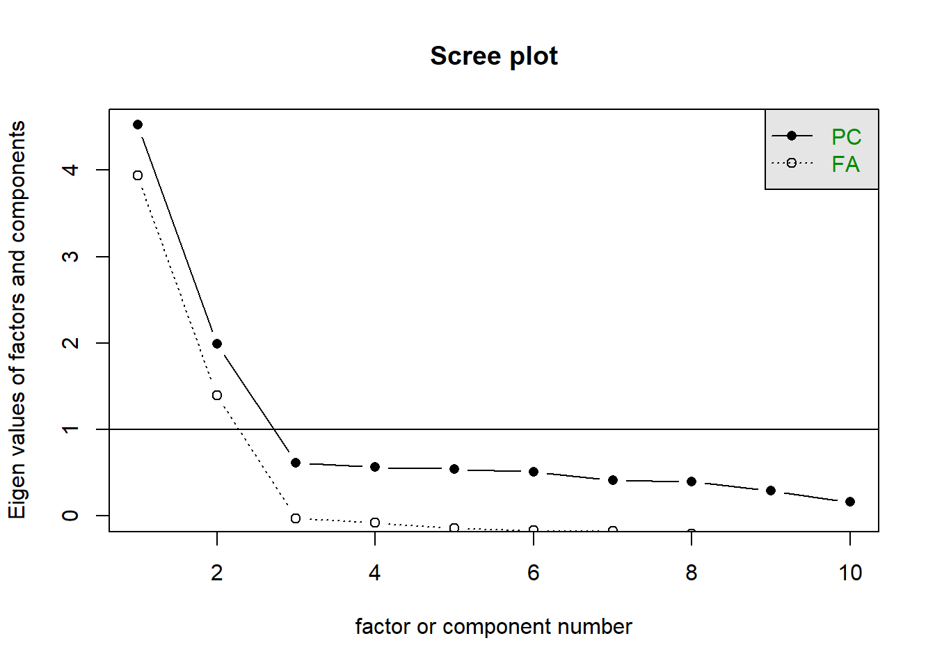
How many dimensions should be retained?

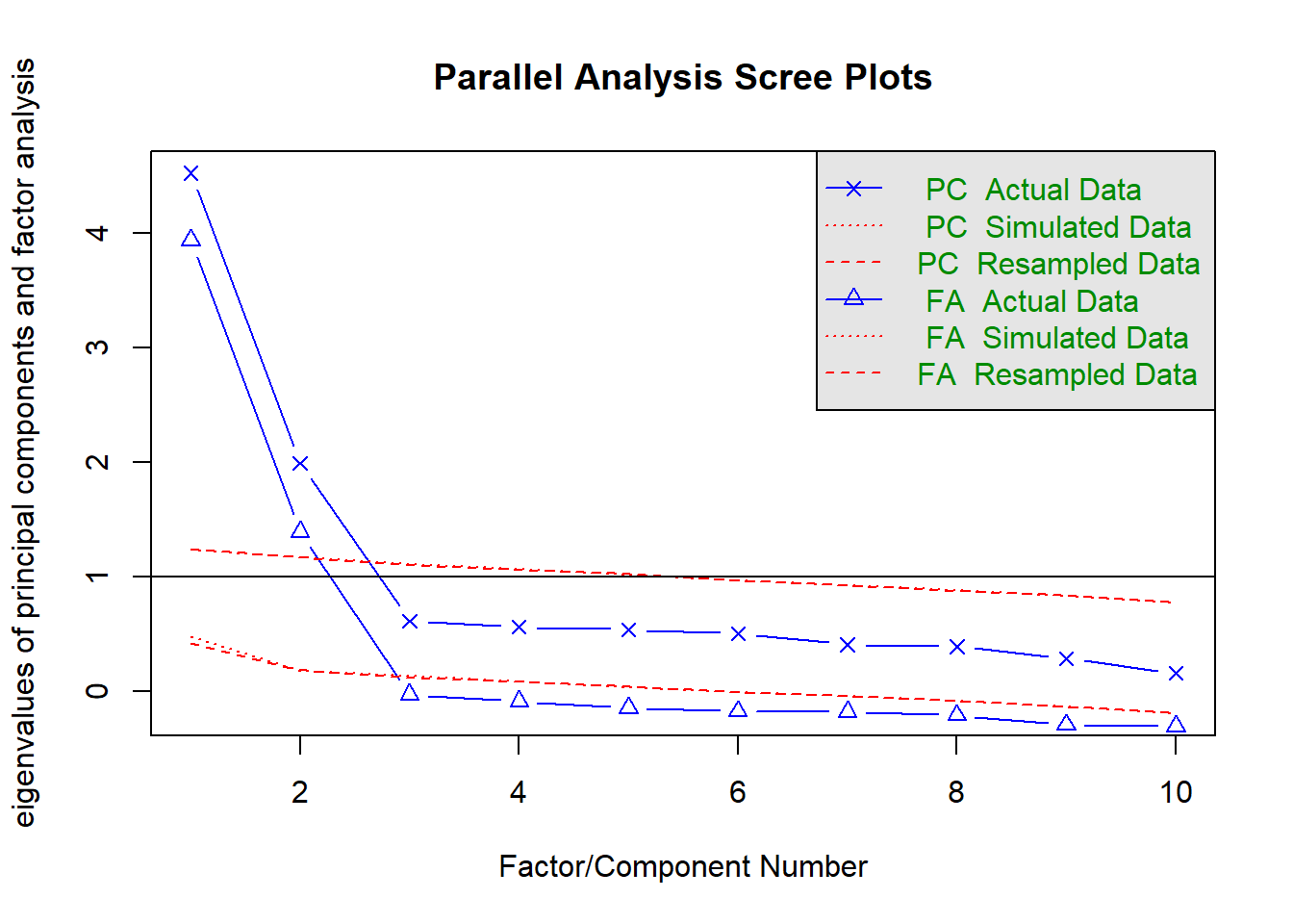
This question can be answered in the same way as we did above for PCA - use a scree plot, parallel analysis, and MAP test to guide you.

You can use fa.parallel(data, fa = "both") to conduct both parallel analysis and view the scree plot!

Solution 12. The scree plot shows a kink at 3, which suggests retaining 2 components.

scree(cpdata)

Solution 13. The MAP suggests retaining 2 factors. I’m just extracting the actuall map values here to save having to show all the other output. We can see that the 2nd entry is the smallest:

VSS(cpdata, plot = FALSE, n = ncol(cpdata))$map

 [1] 0.10575332 0.03377130 0.05762202 0.10352974 0.14935664 0.25195168
 [7] 0.39743503 0.45518643 1.00000000         NA

Solution 14. Parallel analysis suggests 2 factors as well:

fa.parallel(cpdata, fa = "both")

Parallel analysis suggests that the number of factors =  2  and the number of components =  2 

Solution 15. Again, a quite clear picture that 2 factors is preferred:

guides	suggestion
Scree	2
MAP	2
Parallel Analysis	2

Question 9

Use the function fa() from the psych package to conduct and EFA to extract 2 factors (this is what we suggest based on the various tests above, but you might feel differently - the ideal number of factors is subjective!). Use a suitable rotation (rotate = ?) and extraction method (fm = ?).

myfa <- fa(data, nfactors = ?, rotate = ?, fm = ?)

Hints

Would you expect factors to be correlated? If so, you’ll want an oblique rotation.

If there are two+ underlying factors of ‘conduct problems’, if someone is higher on one of them, would we expect them to therefore be high/low on the other? If so, then we the two factors are correlated!

Solution 16. For example, you could choose an oblimin rotation to allow factors to correlate and use ml as the extraction method.

conduct_efa <- fa(cpdata, nfactors=2, rotate='oblimin', fm="ml")

Question 10

Inspect your solution. Make sure to look at and think about the loadings, the variance accounted for, and the factor correlations (if estimated).

What we’re doing here is essentially evaluating whether our solution looks theoretically coherent. A big part of this is a subjective decision about the groupings of items, but we would also like the numerical parts of our model to meet certain criteria (see Chapter 3: EFA#what-makes-a-good-factor-solution).

Hints

Just printing an fa object:

myfa <- fa(data, ..... )
myfa

Will give you lots and lots of information.
You can extract individual parts using:

• myfa$loadings for the loadings
• myfa$Vaccounted for the variance accounted for by each factor
• myfa$Phi for the factor correlation matrix

You can find a quick guide to reading the fa output here: efa_output.pdf.

Solution 17. Things look pretty good here. Each item has a clear primary loading on to one of the factors, and the complexity for all items is 1 (meaning they’re clearly link to just one of the factors). The h2 column is showing that the 2 factor solution is explaining 38%+ of the variance in each item. Both factors are well determined, having at least 3 salient loadings.

The 2 factors together explain 57% of the variance in the data - both factors explain a similar amount (29% for factor 1, 28% for factor 2).

We can also see that there is a moderate correlation between the two factors. Use of an oblique rotation was appropriate - if the correlation had been very weak, then it might not have differed much from if we used an orthogonal rotation.

conduct_efa

Factor Analysis using method =  ml
Call: fa(r = cpdata, nfactors = 2, rotate = "oblimin", fm = "ml")
Standardized loadings (pattern matrix) based upon correlation matrix
                     ML1   ML2   h2   u2 com
breaking_curfew    -0.05  0.88 0.74 0.26   1
vandalism           0.05  0.69 0.51 0.49   1
skipping_school    -0.01  0.67 0.44 0.56   1
bullying            0.90  0.00 0.81 0.19   1
spreading_rumours   0.93 -0.02 0.85 0.15   1
fighting            0.65 -0.02 0.42 0.58   1
lying               0.02  0.77 0.60 0.40   1
using_weapon        0.63  0.09 0.45 0.55   1
stealing            0.04  0.70 0.51 0.49   1
threatening_others  0.62 -0.01 0.38 0.62   1

                       ML1  ML2
SS loadings           2.91 2.80
Proportion Var        0.29 0.28
Cumulative Var        0.29 0.57
Proportion Explained  0.51 0.49
Cumulative Proportion 0.51 1.00

 With factor correlations of 
     ML1  ML2
ML1 1.00 0.43
ML2 0.43 1.00

Mean item complexity =  1

Question 11

Look back to the description of the items, and suggest a name for your factors based on the patterns of loadings.

Hints

To sort the loadings, you can use

print(myfa$loadings, sort = TRUE)

Solution 18. You can inspect the loadings using:

print(conduct_efa$loadings, sort=TRUE)

Loadings:
                   ML1    ML2   
bullying            0.899       
spreading_rumours   0.931       
fighting            0.653       
using_weapon        0.629       
threatening_others  0.621       
breaking_curfew            0.878
vandalism                  0.694
skipping_school            0.671
lying                      0.767
stealing                   0.696

                 ML1   ML2
SS loadings    2.890 2.782
Proportion Var 0.289 0.278
Cumulative Var 0.289 0.567

We can see that, ordered like this, we have five items that have high loadings for one factor and another five items that have high loadings for the other.

The five items for factor 1 all have in common that they are non-aggressive forms of conduct problems. The five items for factor 2 are all more aggressive behaviours. We could, therefore, label our factors: ‘non-aggressive’ and ‘aggressive’ conduct problems.

Question 12

Compare your three different solutions:

1. your current solution from the previous questions
2. one where you fit 1 more factor
3. one where you fit 1 fewer factors

Which one looks best?

Hints

We’re looking here to assess:

• how much variance is accounted for by each solution
• do all factors load on 3+ items at a salient level?
  
• do all items have at least one loading at a salient level?
• are there any “Heywood cases” (communalities or standardised loadings that are >1)?
• should we perhaps remove some of the more complex items?
• is the factor structure (items that load on to each factor) coherent, and does it make theoretical sense?

Solution 19. The 1-factor model explains 37% of the variance (as opposed to the 57% explained by the 2 factor solution), and all items load fairly high on the factor. The downside here is that we’re not discerning between different types of conduct problems that we did in the 2 factor solution.

conduct_1 <- fa(cpdata, nfactors=1, fm="ml")
conduct_1

Factor Analysis using method =  ml
Call: fa(r = cpdata, nfactors = 1, fm = "ml")
Standardized loadings (pattern matrix) based upon correlation matrix
                    ML1   h2   u2 com
breaking_curfew    0.42 0.18 0.82   1
vandalism          0.42 0.18 0.82   1
skipping_school    0.35 0.13 0.87   1
bullying           0.89 0.79 0.21   1
spreading_rumours  0.90 0.81 0.19   1
fighting           0.64 0.41 0.59   1
lying              0.43 0.18 0.82   1
using_weapon       0.68 0.46 0.54   1
stealing           0.42 0.17 0.83   1
threatening_others 0.61 0.38 0.62   1

                ML1
SS loadings    3.69
Proportion Var 0.37

Mean item complexity =  1
Test of the hypothesis that 1 factor is sufficient.

df null model =  45  with the objective function =  5.03 with Chi Square =  2237.53
df of  the model are 35  and the objective function was  1.78 

The root mean square of the residuals (RMSR) is  0.19 
The df corrected root mean square of the residuals is  0.22 

The harmonic n.obs is  450 with the empirical chi square  1464.73  with prob <  1.9e-285 
The total n.obs was  450  with Likelihood Chi Square =  789.3  with prob <  3.4e-143 

Tucker Lewis Index of factoring reliability =  0.557
RMSEA index =  0.219  and the 90 % confidence intervals are  0.206 0.232
BIC =  575.48
Fit based upon off diagonal values = 0.8
Measures of factor score adequacy             
                                                   ML1
Correlation of (regression) scores with factors   0.96
Multiple R square of scores with factors          0.92
Minimum correlation of possible factor scores     0.84

The 3-factor model explains 60% of the variance (only 3% more than the 2-factor model). Notably, the third factor is not very clearly defined - it only has 1 salient loading (possibly 2 if we consider the 0.31 to be salient, but that item is primarily loaded on the 2nd factor).

conduct_3 <- fa(cpdata, nfactors=3, rotate='oblimin', fm="ml")
conduct_3

Factor Analysis using method =  ml
Call: fa(r = cpdata, nfactors = 3, rotate = "oblimin", fm = "ml")
Standardized loadings (pattern matrix) based upon correlation matrix
                     ML1   ML2   ML3   h2   u2 com
breaking_curfew    -0.02  0.61  0.31 0.71 0.29 1.5
vandalism           0.06  0.12  0.74 0.72 0.28 1.1
skipping_school     0.00  0.56  0.14 0.44 0.56 1.1
bullying            0.90  0.09 -0.10 0.82 0.18 1.0
spreading_rumours   0.92 -0.02  0.03 0.85 0.15 1.0
fighting            0.65 -0.13  0.14 0.43 0.57 1.2
lying               0.02  0.85 -0.06 0.67 0.33 1.0
using_weapon        0.63  0.08  0.02 0.45 0.55 1.0
stealing            0.06  0.69  0.02 0.53 0.47 1.0
threatening_others  0.62 -0.08  0.09 0.39 0.61 1.1

                       ML1  ML2  ML3
SS loadings           2.93 2.14 0.94
Proportion Var        0.29 0.21 0.09
Cumulative Var        0.29 0.51 0.60
Proportion Explained  0.49 0.36 0.16
Cumulative Proportion 0.49 0.84 1.00

 With factor correlations of 
     ML1  ML2  ML3
ML1 1.00 0.39 0.32
ML2 0.39 1.00 0.68
ML3 0.32 0.68 1.00

Mean item complexity =  1.1
Test of the hypothesis that 3 factors are sufficient.

df null model =  45  with the objective function =  5.03 with Chi Square =  2237.53
df of  the model are 18  and the objective function was  0.02 

The root mean square of the residuals (RMSR) is  0.01 
The df corrected root mean square of the residuals is  0.02 

The harmonic n.obs is  450 with the empirical chi square  3.98  with prob <  1 
The total n.obs was  450  with Likelihood Chi Square =  10.51  with prob <  0.91 

Tucker Lewis Index of factoring reliability =  1.009
RMSEA index =  0  and the 90 % confidence intervals are  0 0.016
BIC =  -99.46
Fit based upon off diagonal values = 1
Measures of factor score adequacy             
                                                   ML1  ML2  ML3
Correlation of (regression) scores with factors   0.96 0.93 0.88
Multiple R square of scores with factors          0.93 0.86 0.77
Minimum correlation of possible factor scores     0.85 0.72 0.53

Question 13

Drawing on your previous answers and conducting any additional analyses you believe would be necessary to identify an optimal factor structure for the 10 conduct problems, write some bullet points to summarise your methods and the results of your chosen optimal model.

Remember, the main principles governing the reporting of statistical methods are transparency and reproducibility (i.e., someone should be able to reproduce your analysis based on your description).

Solution 20. An example summary would be:

First, the data were checked for their suitability for factor analysis. Normality was checked using visual inspection of histograms, linearity was checked through the inspection of the linear and lowess lines for the pairwise relations of the variables, and factorability was confirmed using a KMO test, which yielded an overall KMO of \(.87\) with no variable KMOs \(<.50\). An exploratory factor analysis was conducted to inform the structure of a new conduct problems test. Inspection of a scree plot alongside parallel analysis (using principal components analysis; PA-PCA) and the MAP test were used to guide the number of factors to retain. All three methods suggested retaining two factors; however, a one-factor and three-factor solution were inspected to confirm that the two-factor solution was optimal from a substantive and practical perspective, e.g., that it neither blurred important factor distinctions nor included a minor factor that would be better combined with the other in a one-factor solution. These factor analyses were conducted using maximum likelihood estimation and (for the two- and three-factor solutions) an oblimin rotation, because it was expected that the factors would correlate. Inspection of the factor loadings and correlations reinforced that the two-factor solution was optimal: both factors were well-determined, including 5 loadings \(>|0.3|\) and the one-factor model blurred the distinction between different forms of conduct problems. The factor loadings are provided in Table 2¹. Based on the pattern of factor loadings, the two factors were labelled ‘aggressive conduct problems’ and ‘non-aggressive conduct problems’. These factors had a correlation of \(r=.43\). Overall, they accounted for 57% of the variance in the items, suggesting that a two-factor solution effectively summarised the over half of the variation in the items.

                     ML1   ML2
spreading_rumours  0.931    NA
bullying           0.899    NA
fighting           0.653    NA
using_weapon       0.629    NA
threatening_others 0.621    NA
vandalism             NA 0.694
stealing              NA 0.696
lying                 NA 0.767
skipping_school       NA 0.671
breaking_curfew       NA 0.878

Table 2: Factor Loadings

	ML1	ML2
spreading_rumours	0.93
bullying	0.90
fighting	0.65
using_weapon	0.63
threatening_others	0.62
vandalism		0.69
stealing		0.70
lying		0.77
skipping_school		0.67
breaking_curfew		0.88

Footnotes

1. You should provide the table of factor loadings. It is conventional to omit factor loadings \(<|0.3|\); however, be sure to ensure that you mention this in a table note.