DAPR3 Lab Exercises
  • Linear mixed models
    • Identifying grouping structure
    • Modelling group-level variability using random effects
    • Building maximal models and interpreting LMM estimates
    • Troubleshooting, checking assumptions and diagnostics
    • LMMs: Practice write-up
  • Measurement & Dimension Reduction
    • Scale Scores & PCA
    • EFA
    • CFA
  • Week 11: Mock Exam SAQs

CFA

Get set up
  1. Create a new .Rmd file for this week’s exercises.
  2. Save it somewhere you can find it again.
  3. Give it a clear name (for example, dapr3_lab09.Rmd).
  4. In the first code chunk, load the packages you’ll need this week:
    • tidyverse
    • lavaan
    • semPlot

Quality Street

Our exercises today are concerning the factor structure of the “WHOQOL-BREF” - a brief measure of quality of life developed by the World Health Organisation (WHO). It contains 26 questions (the first two of which are treated individually as general single item measures). The remaining 24 questions captures four related aspects of quality of life: Physical, Psychological, Social and Environmental.

In practice, these four domain scores are often highly correlated (\(r > .70\)). Researcher A is curious about whether this scale is genuinely measuring four distinct domains or simply reflecting one underlying construct (a “General Quality of Life”). She wants to test whether a complex 4-factor structure is strictly necessary to explain the responses, or whether a simpler 1-factor model is sufficient. She collects WHOQOL-BREF data from 300 adults aged 25 to 55.
The wordings of the items can be found below.
The dataset can be accessed at https://uoepsy.github.io/data/whoqolbref-sampleA.csv

Item Wordings
q domain wording
q1 NA How would you rate your quality of life?
q2 NA How satisfied are you with your health?
q3 Physical To what extent do you feel that (physical) pain prevents you from doing what you need to do?
q4 Physical How much do you need any medical treatment to function in your daily life?
q5 Psychological How much do you enjoy life?
q6 Psychological To what extent do you feel your life to be meaningful?
q7 Psychological How well are you able to concentrate?
q8 Environmental How safe do you feel in your daily life?
q9 Environmental How healthy is your physical environment?
q10 Physical Do you have enough energy for everyday life?
q11 Psychological Are you able to accept your bodily appearance?
q12 Environmental Have you enough money to meet your needs?
q13 Environmental How available to you is the information that you need in your day-to-day life?
q14 Environmental To what extent do you have the opportunity for leisure activities?
q15 Physical How well are you able to get around?
q16 Physical How satisfied are you with your sleep?
q17 Physical How satisfied are you with your ability to perform your daily living activities?
q18 Physical How satisfied are you with your capacity for work?
q19 Psychological How satisfied are you with yourself?
q20 Social How satisfied are you with your personal relationships?
q21 Social How satisfied are you with your sex life?
q22 Social How satisfied are you with the support you get from your friends?
q23 Environmental How satisfied are you with the conditions of your living place?
q24 Environmental How satisfied are you with your access to health services?
q25 Environmental How satisfied are you with your transport?
q26 Psychological How often do you have negative feelings such as blue mood, despair, anxiety, depression?
Question 1

First, let’s work with the factor model that is suggested by the WHO. We can then see if this factor structure provides a good fit to the responses from our sample.

In the syntax for lavaan, specify the model. (We need to specify the model that links the specific questions to their relevant “domains”)

who_mod <- "
    ...
    ...
    
    ...
  "

🗂️ See the #Specification section on the Fit a Confirmatory Factor Model flash card.

Solution 1.

who_mod <- '
  Phys =~ q3 + q4 + q10 + q15 + q16 + q17 + q18
  Psych =~ q5 + q6 + q7 + q11 + q19 + q26
  Social =~ q20 + q21 + q22
  Env =~ q8 + q9 + q12 + q13 + q14 + q23 + q24 + q25
'

Question 2

Fit the model, and evaluate the global (overall) model fit.

🗂️ See the #Estimation section on the Fit a Confirmatory Factor Model flash card.

Solution 2.

whqb_a <- read_csv("https://uoepsy.github.io/data/whoqolbref-sampleA.csv")

fit_who <- cfa(who_mod, data = whqb_a, std.lv = TRUE)

fitmeasures(fit_who)[c("rmsea","srmr","cfi","tli")]
 rmsea   srmr    cfi    tli 
0.0244 0.0416 0.9766 0.9738 

Question 3

Examine the modification indices.
Even if the model already “fits well”, this can help to highlight possible issues with the measurement instrument.
What might large residual covariances between two items tell us?

🗂️ See the #Re-specification section on the Fit a Confirmatory Factor Model flash card.

Hints

This will require looking carefully at the item wordings. What do the items with suggested residual covariances all have in common?

Solution 3.

modindices(fit_who, sort = TRUE) |> 
  head(5)
    lhs op rhs    mi   epc sepc.lv sepc.all sepc.nox
142  q3 ~~ q26 19.49 0.129   0.129    0.286    0.286
164  q4 ~~ q26 19.33 0.126   0.126    0.283    0.283
131  q3 ~~  q4 13.53 0.119   0.119    0.258    0.258
167  q4 ~~ q22  9.29 0.110   0.110    0.202    0.202
375 q22 ~~ q14  9.02 0.125   0.125    0.198    0.198

You might notice that these top 3 - questions q3, q4, q26 - are the only negatively worded questions! Respondents often process negatively framed items with their specific cognitive bias that can creating residual correlation among them. But this is more noise due to the method than theoretically interesting domain variability.

Question 4

When you fitted your model, which did you use?

cfa(model, data)
cfa(model, data, std.lv = TRUE)

To help us better understand how this changes things, fit the other one now, and examine what (if anything) is different.

  • global fit of the model
  • modification indices
  • in summary():
    • factor loading estimates (the Estimate column under the “Latent Variables” section)
    • factor covariance estimates (the Estimate column under the “Covariances” section)

Bonus Challenge: can you see the link between estimates from the two versions?

🗂️ See the #Parameter Estimates section on the Fit a Confirmatory Factor Model flash card.

Solution 4.

with std.lv = TRUE

fit_who <- cfa(who_mod, data = whqb_a, std.lv = TRUE)
summary(fit_who)
lavaan 0.7-3 ended normally after 21 iterations

  Estimator                                         ML
  Optimization method                           NLMINB
  Number of model parameters                        54

  Number of observations                           300

Model Test User Model:
                                                      
  Test statistic                               289.832
  Degrees of freedom                               246
  P-value (Chi-square)                           0.029
                                                      
  Browne's residual (NT model-based) test             
  Test statistic                               288.292
  Degrees of freedom                               246
  P-value (Chi-square)                           0.033

Parameter Estimates:

  Standard errors                             Standard
  Information                                 Expected
  Information saturated (h1) model          Structured

Latent Variables:
                   Estimate  Std.Err  z-value  P(>|z|)
  Phys =~                                             
    q3                0.623    0.051   12.297    0.000
    q4                0.584    0.049   11.865    0.000
    q10              -0.475    0.041  -11.682    0.000
    q15              -0.600    0.059  -10.198    0.000
    q16              -0.657    0.059  -11.156    0.000
    q17              -0.585    0.049  -11.932    0.000
    q18              -0.517    0.042  -12.202    0.000
  Psych =~                                            
    q5                0.555    0.049   11.348    0.000
    q6                0.596    0.052   11.392    0.000
    q7                0.632    0.054   11.700    0.000
    q11               0.502    0.056    8.940    0.000
    q19               0.564    0.048   11.640    0.000
    q26              -0.457    0.047   -9.802    0.000
  Social =~                                           
    q20               0.576    0.064    8.943    0.000
    q21               0.489    0.057    8.556    0.000
    q22               0.510    0.066    7.770    0.000
  Env =~                                              
    q8                0.674    0.051   13.164    0.000
    q9                0.560    0.054   10.356    0.000
    q12               0.492    0.051    9.582    0.000
    q13               0.401    0.043    9.333    0.000
    q14               0.628    0.057   11.094    0.000
    q23               0.641    0.056   11.446    0.000
    q24               0.419    0.047    8.891    0.000
    q25               0.433    0.053    8.212    0.000

Covariances:
                   Estimate  Std.Err  z-value  P(>|z|)
  Phys ~~                                             
    Psych            -0.639    0.048  -13.181    0.000
    Social           -0.428    0.072   -5.980    0.000
    Env              -0.534    0.054   -9.883    0.000
  Psych ~~                                            
    Social            0.441    0.073    6.030    0.000
    Env               0.573    0.054   10.707    0.000
  Social ~~                                           
    Env               0.485    0.070    6.950    0.000

Variances:
                   Estimate  Std.Err  z-value  P(>|z|)
   .q3                0.469    0.045   10.439    0.000
   .q4                0.455    0.043   10.612    0.000
   .q10               0.314    0.029   10.680    0.000
   .q15               0.712    0.064   11.147    0.000
   .q16               0.679    0.062   10.862    0.000
   .q17               0.450    0.043   10.586    0.000
   .q18               0.330    0.031   10.479    0.000
   .q5                0.438    0.042   10.337    0.000
   .q6                0.500    0.048   10.317    0.000
   .q7                0.522    0.051   10.167    0.000
   .q11               0.655    0.058   11.209    0.000
   .q19               0.421    0.041   10.197    0.000
   .q26               0.434    0.040   10.947    0.000
   .q20               0.521    0.065    7.973    0.000
   .q21               0.442    0.051    8.601    0.000
   .q22               0.649    0.068    9.588    0.000
   .q8                0.434    0.045    9.674    0.000
   .q9                0.582    0.053   10.928    0.000
   .q12               0.545    0.049   11.161    0.000
   .q13               0.385    0.034   11.228    0.000
   .q14               0.613    0.057   10.669    0.000
   .q23               0.587    0.056   10.530    0.000
   .q24               0.473    0.042   11.340    0.000
   .q25               0.607    0.053   11.494    0.000
    Phys              1.000                           
    Psych             1.000                           
    Social            1.000                           
    Env               1.000                           

without std.lv = TRUE

fit_who2 <- cfa(who_mod, data = whqb_a)
summary(fit_who2)
lavaan 0.7-3 ended normally after 42 iterations

  Estimator                                         ML
  Optimization method                           NLMINB
  Number of model parameters                        54

  Number of observations                           300

Model Test User Model:
                                                      
  Test statistic                               289.832
  Degrees of freedom                               246
  P-value (Chi-square)                           0.029
                                                      
  Browne's residual (NT model-based) test             
  Test statistic                               288.291
  Degrees of freedom                               246
  P-value (Chi-square)                           0.033

Parameter Estimates:

  Standard errors                             Standard
  Information                                 Expected
  Information saturated (h1) model          Structured

Latent Variables:
                   Estimate  Std.Err  z-value  P(>|z|)
  Phys =~                                             
    q3                1.000                           
    q4                0.937    0.096    9.734    0.000
    q10              -0.762    0.079   -9.634    0.000
    q15              -0.963    0.110   -8.754    0.000
    q16              -1.054    0.113   -9.335    0.000
    q17              -0.940    0.096   -9.771    0.000
    q18              -0.829    0.084   -9.915    0.000
  Psych =~                                            
    q5                1.000                           
    q6                1.075    0.120    8.976    0.000
    q7                1.139    0.125    9.121    0.000
    q11               0.905    0.119    7.632    0.000
    q19               1.016    0.112    9.093    0.000
    q26              -0.824    0.101   -8.143    0.000
  Social =~                                           
    q20               1.000                           
    q21               0.849    0.138    6.141    0.000
    q22               0.885    0.149    5.923    0.000
  Env =~                                              
    q8                1.000                           
    q9                0.831    0.091    9.128    0.000
    q12               0.730    0.085    8.588    0.000
    q13               0.595    0.071    8.408    0.000
    q14               0.933    0.097    9.615    0.000
    q23               0.952    0.097    9.838    0.000
    q24               0.622    0.077    8.082    0.000
    q25               0.643    0.085    7.563    0.000

Covariances:
                   Estimate  Std.Err  z-value  P(>|z|)
  Phys ~~                                             
    Psych            -0.221    0.035   -6.326    0.000
    Social           -0.153    0.034   -4.453    0.000
    Env              -0.224    0.037   -5.984    0.000
  Psych ~~                                            
    Social            0.141    0.032    4.430    0.000
    Env               0.214    0.035    6.053    0.000
  Social ~~                                           
    Env               0.188    0.039    4.875    0.000

Variances:
                   Estimate  Std.Err  z-value  P(>|z|)
   .q3                0.469    0.045   10.439    0.000
   .q4                0.455    0.043   10.612    0.000
   .q10               0.314    0.029   10.680    0.000
   .q15               0.712    0.064   11.147    0.000
   .q16               0.679    0.062   10.862    0.000
   .q17               0.450    0.043   10.586    0.000
   .q18               0.330    0.031   10.479    0.000
   .q5                0.438    0.042   10.337    0.000
   .q6                0.500    0.048   10.317    0.000
   .q7                0.522    0.051   10.167    0.000
   .q11               0.655    0.058   11.209    0.000
   .q19               0.421    0.041   10.197    0.000
   .q26               0.434    0.040   10.947    0.000
   .q20               0.521    0.065    7.973    0.000
   .q21               0.442    0.051    8.601    0.000
   .q22               0.649    0.068    9.588    0.000
   .q8                0.434    0.045    9.674    0.000
   .q9                0.582    0.053   10.928    0.000
   .q12               0.545    0.049   11.161    0.000
   .q13               0.385    0.034   11.228    0.000
   .q14               0.613    0.057   10.669    0.000
   .q23               0.587    0.056   10.530    0.000
   .q24               0.473    0.042   11.340    0.000
   .q25               0.607    0.053   11.494    0.000
    Phys              0.388    0.063    6.149    0.000
    Psych             0.308    0.054    5.674    0.000
    Social            0.331    0.074    4.472    0.000
    Env               0.454    0.069    6.582    0.000

Solution 5.

fit_who <- cfa(who_mod, data = whqb_a, std.lv = TRUE)
fit_who2 <- cfa(who_mod, data = whqb_a)

The fit of the models should be identical:

fitmeasures(fit_who)[c("rmsea","srmr","cfi","tli")]
 rmsea   srmr    cfi    tli 
0.0244 0.0416 0.9766 0.9738 
fitmeasures(fit_who2)[c("rmsea","srmr","cfi","tli")]
 rmsea   srmr    cfi    tli 
0.0244 0.0416 0.9766 0.9738 

And the modification indices should also be indentical:

head(modindices(fit_who, sort = TRUE))
    lhs op rhs    mi   epc sepc.lv sepc.all sepc.nox
142  q3 ~~ q26 19.49 0.129   0.129    0.286    0.286
164  q4 ~~ q26 19.33 0.126   0.126    0.283    0.283
131  q3 ~~  q4 13.53 0.119   0.119    0.258    0.258
167  q4 ~~ q22  9.29 0.110   0.110    0.202    0.202
375 q22 ~~ q14  9.02 0.125   0.125    0.198    0.198
185 q10 ~~ q26  8.76 0.070   0.070    0.190    0.190
head(modindices(fit_who2, sort = TRUE))
    lhs op rhs    mi   epc sepc.lv sepc.all sepc.nox
142  q3 ~~ q26 19.49 0.129   0.129    0.286    0.286
164  q4 ~~ q26 19.33 0.126   0.126    0.283    0.283
131  q3 ~~  q4 13.53 0.119   0.119    0.258    0.258
167  q4 ~~ q22  9.29 0.110   0.110    0.202    0.202
375 q22 ~~ q14  9.02 0.125   0.125    0.198    0.198
185 q10 ~~ q26  8.76 0.070   0.070    0.190    0.190

The loadings will be different.

  • without std.lv = TRUE, the first loading is fixed to 1, and all the others are in comparison to that one
  • with std.lv = TRUE, the loadings are all freely estimated but the latent variable has a variance of 1

For instance, the items loading on the social domain have these loadings when we use std.lv = TRUE: 0.576, 0.489, 0.510.
And when we don’t use it, we get: 1.000, 0.849, 0.885.

To see how they match up:

c(0.576, 0.489, 0.510) / 0.576
[1] 1.000 0.849 0.885

The factor covariances are also different.

  • without std.lv = TRUE, they are covariances between latent variables that have scales fixed to the same as their first item. covariances are dependent on units, remember!
  • with std.lv = TRUE, the latent variables have variances of 1, so they are all standardised. so covariances become correlations!

Question 5

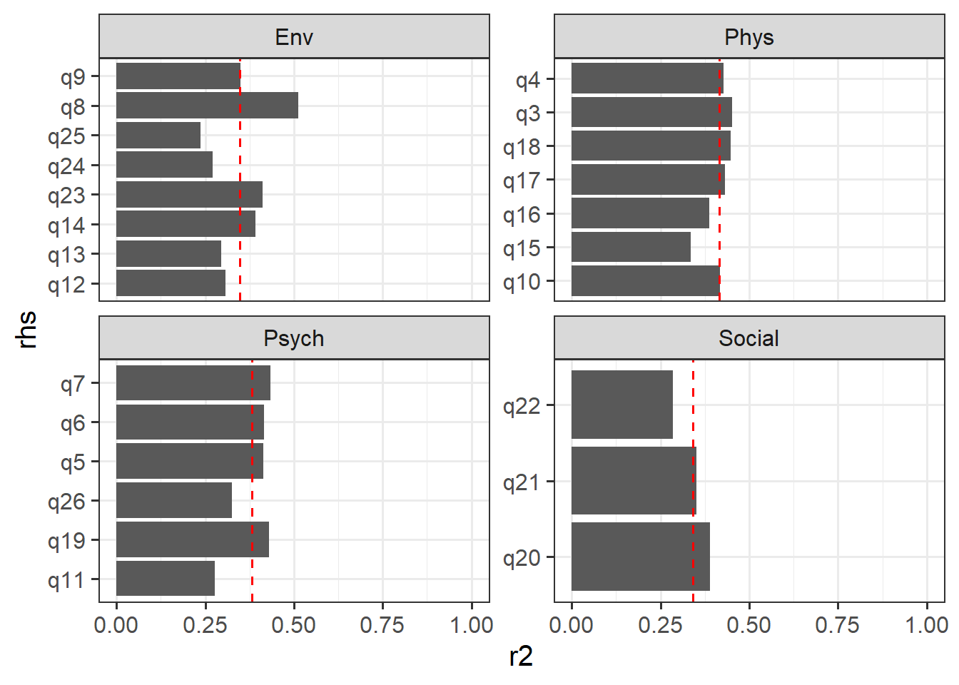
How do the individual items look? How much variance in each item is explained by its corresponding factor?

Bonus Challenge: Can you calculate the “average variance explained” for each factor?

Hints

When we have a standardised factor loading, it is just like EFA, where squaring it gives the variance in an item explained by a factor.

Solution 6. I love making plots rather than looking at numbers, so here we go!

standardizedsolution(fit_who) |>
  filter(op == "=~") |>
  mutate(r2 = est.std^2) |>
  group_by(lhs) |>
  mutate(mean_r2 = mean(r2)) |>
  ggplot(aes(x = rhs, y = r2)) +
  geom_col() +
  geom_hline(aes(yintercept = mean_r2),
             linetype = "dashed", color = "red") +
  ylim(0,1)+
  coord_flip() + 
  facet_wrap(~lhs, scales = "free_y") 

Question 6

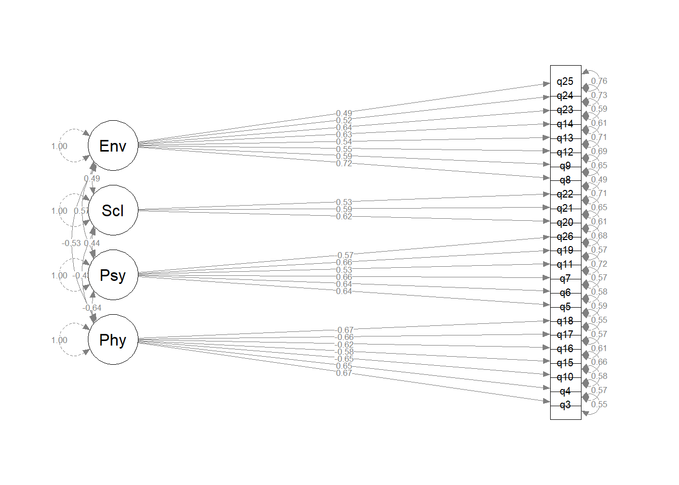
Make a quick diagram showing the standardised loadings for each factor.

🗂️ See the #Drawing your fitted model section on the Fit a Confirmatory Factor Model flash card.

Solution 7.

library(semPlot)

semPaths(fit_who, whatLabels = "std", rotation=2)

Question 7

Researcher A would now like to compare this to a model with only one single factor.

Fit a unidimensional model and compare the fit measures.

Solution 8.

rA_mod <- '
  GQOL =~ q3 + q4 + q10 + q15 + q16 + q17 + q18 + q5 + q6 + q7 + q11 + q19 + q26 + q20 + q21 + q22 + q8 + q9 + q12 + q13 + q14 + q23 + q24 + q25
'

fit_a <- cfa(rA_mod, whqb_a, std.lv=TRUE)
fitmeasures(fit_a)[c("rmsea","srmr","cfi","tli")]
 rmsea   srmr    cfi    tli 
0.0794 0.0774 0.7459 0.7216 

Quality over Quantity

Researcher B is working on the same project, and wonders whether this factor structure holds up across different age demographics. Specifically, he wants to ask if the optimal factor structure identified in younger adults (25–55) holds true in older adults aged 65+? Is the WHOQOL-BREF measurement “invariant” across these two age groups, or do older adults interpret and answer the items differently?
To test this, Researcher B recruits a second sample of 300 adults aged 65 and above who complete the same 26 items.

The data are available at https://uoepsy.github.io/data/whoqolbref-sampleB.csv

Question 8

Fit the WHO 4 factor model to sample B (the sample of 300 adults >65).

Does it fit well?

Solution 9.

whqb_b <- read_csv("https://uoepsy.github.io/data/whoqolbref-sampleB.csv")

fit_bwho <- cfa(who_mod, whqb_b, std.lv = TRUE)

fitmeasures(fit_bwho)[c("rmsea","srmr","cfi","tli")]
 rmsea   srmr    cfi    tli 
0.0322 0.0505 0.9469 0.9404 

Question 9

Compare the loadings of the models fitted to the 25-55 year old sample and the 65+ sample.
Can you make any suggestions on why certain items might mean different things to these two groups?

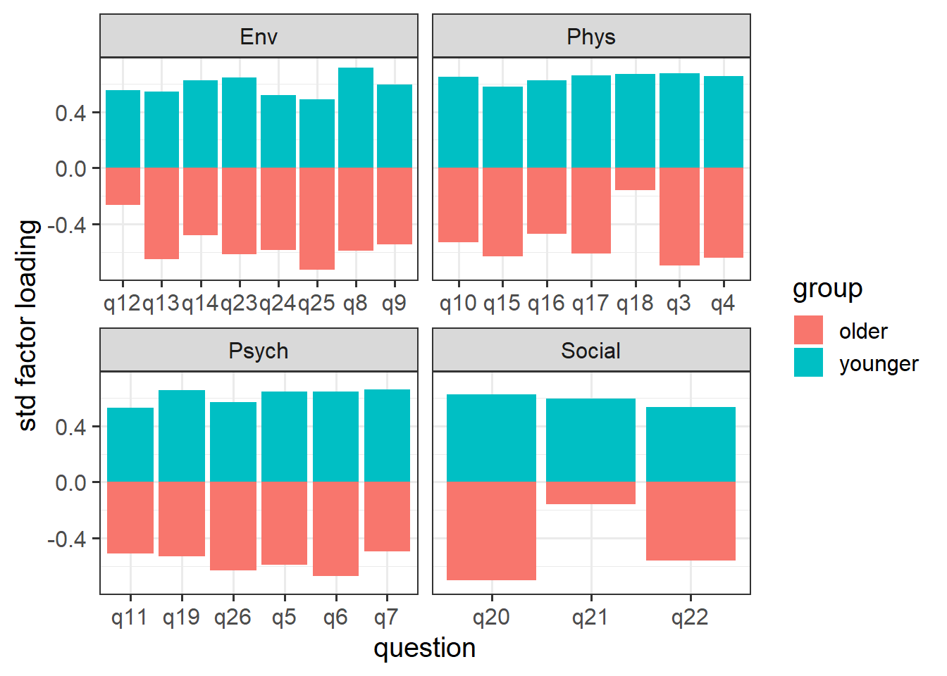
Solution 10. We can look through summary() or standardizedsolution() for each model and just compare the various numbers. Or we could draw diagrams for both models using semPaths() and compare.

However, i’m going to plot stuff again (you don’t have to, i just prefer it!).

What does it tell us? it looks like loadings for q12, q18, and q21 specifically are quite a lot weaker than in the younger group. And some questions (q25) are a bit higher!

wqit |> 
  filter(q %in% c("q12","q18","q21","q25")) |>
  gt::gt()
q domain wording
q12 Environmental Have you enough money to meet your needs?
q18 Physical How satisfied are you with your capacity for work?
q21 Social How satisfied are you with your sex life?
q25 Environmental How satisfied are you with your transport?

This makes a little bit of sense when we think about it. People over the age of 65 are often retired, meaning q18 is kind of irrelevant? And the same reasoning might be said for q21. They might have fewer financial outgoings, making q12 less indicative of quality of life. q25 possibly becomes far more indicative of quality of life because older people will be more likely to be infirm and unable to drive etc.

Question Extra 10

Researcher A, who is happy that the WHOQOL-BREF appears to fit well in her sample of working aged adults, has another question.

Which specific domain is the strongest unique predictor of the single item measure (q1) of an overall quality of life?

She fits the model below.
Can you answer her question?
a2_mod <- '
  # measurement
  Phys =~ q3 + q4 + q10 + q15 + q16 + q17 + q18
  Psych =~ q5 + q6 + q7 + q11 + q19 + q26
  Social =~ q20 + q21 + q22
  Env =~ q8 + q9 + q12 + q13 + q14 + q23 + q24 + q25
  
  # regression
  q1 ~ Phys + Psych + Social + Env
'

fit_a2 <- sem(a2_mod, whqb_a, std.lv = TRUE)

Solution 11.

standardizedsolution(fit_a2) |>
  filter(op == "~") 
  lhs op    rhs est.std    se    z pvalue ci.lower ci.upper
1  q1  ~   Phys   0.436 0.089 4.89  0.000    0.261    0.611
2  q1  ~  Psych   0.378 0.096 3.93  0.000    0.189    0.566
3  q1  ~ Social   0.083 0.090 0.93  0.352   -0.092    0.259
4  q1  ~    Env   0.274 0.087 3.16  0.002    0.104    0.444