EFA

Get set up

1. Create a new .Rmd file for this week’s exercises.
2. Save it somewhere you can find it again.
3. Give it a clear name (for example, dapr3_lab08.Rmd).
4. In the first code chunk, load the packages you’ll need this week:
   • tidyverse
   • psych

---

copingstrats.csv

These data come from the development of a short measure of people’s “coping strategies”.
A sample of 620 people filled in a questionnaire that included 28 self-report items assessing the different ways individuals respond to stress in their daily lives. Participants rated each statement on a 5-point Likert scale ranging from 1 (“I haven’t been doing this at all”) to 5 (“I’ve been doing this a lot”), indicating how frequently they used each specific coping response when facing stressful events.

Study aim: Explore the underlying structure of the 28-item pool and (if necessary) refine the questionnaire into a well-defined measure of distinct coping strategies.

Item Wordings

variable	wording
q1	I've been turning to work or other activities to take my mind off things.
q2	I've been concentrating my efforts on doing something about the situation I'm in.
q3	I've been saying to myself "this isn't real.".
q4	I've been using alcohol or other drugs to make myself feel better.
q5	I've been getting emotional support from others.
q6	I've been giving up trying to deal with it.
q7	I've been taking action to try to make the situation better.
q8	I've been refusing to believe that it has happened.
q9	I've been saying things to let my unpleasant feelings escape.
q10	I've been getting help and advice from other people.
q11	I've been using alcohol or other drugs to help me get through it.
q12	I've been trying to see it in a different light, to make it seem more positive.
q13	I've been criticizing myself.
q14	I've been trying to come up with a strategy about what to do.
q15	I've been getting comfort and understanding from someone.
q16	I've been giving up the attempt to cope.
q17	I've been looking for something good in what is happening.
q18	I've been making jokes about it.
q19	I've been doing something to think about it less, such as going to movies, watching TV, reading, daydreaming, sleeping, or shopping.
q20	I've been accepting the reality of the fact that it has happened.
q21	I've been expressing my negative feelings.
q22	I've been trying to find comfort in my religion or spiritual beliefs.
q23	I've been trying to get advice or help from other people about what to do.
q24	I've been learning to live with it.
q25	I've been thinking hard about what steps to take.
q26	I've been blaming myself for things that happened.
q27	I've been praying or meditating.
q28	I've been making fun of the situation.

Question 1

Read in the data and check the suitability of the items for EFA.

Things to look at: correlation matrix, bartlett’s test, KMO

🗂️ See the Check Suitability for Factor Analysis flash card.

Solution 1.

library(tidyverse)
library(psych)
#bcdata <-read_csv()
copeitems <- bcdata |> select(-pptID)

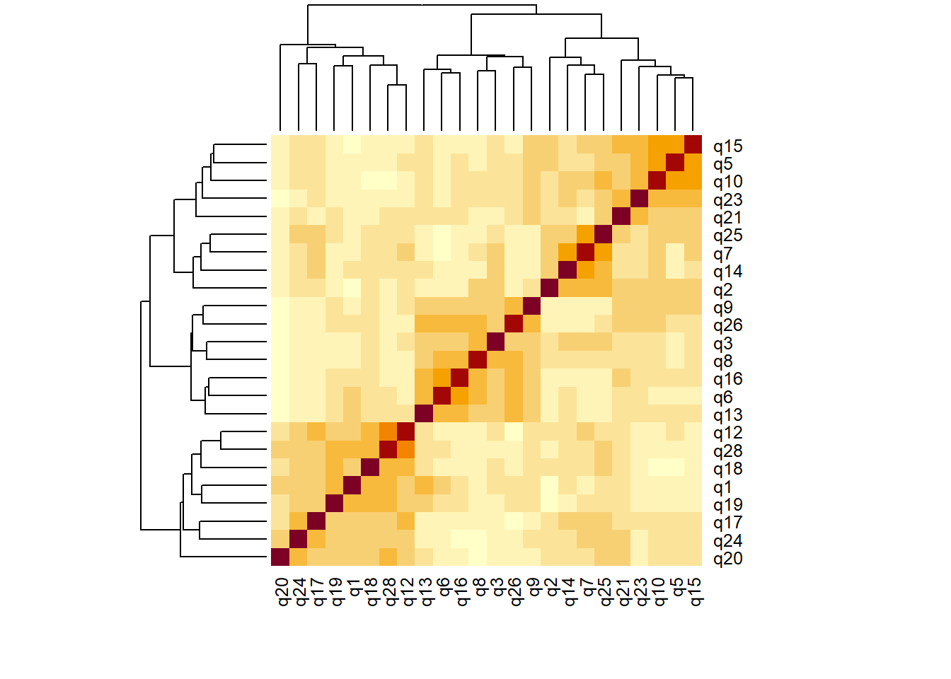
This is too big to look at sensibly as a set of numbers..

cor(copeitems, )

better as an image:

cor(copeitems) |>
  heatmap()

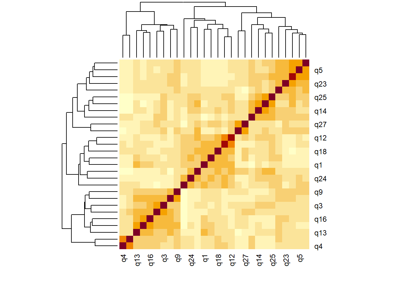
Looks like we have some non-zero correlations!

bartlett.test(copeitems)

    Bartlett test of homogeneity of variances

data:  copeitems
Bartlett's K-squared = 205, df = 27, p-value <2e-16

And KMO, along with individual item KMOs, all seem okay.

KMO(copeitems)

Kaiser-Meyer-Olkin factor adequacy
Call: KMO(r = copeitems)
Overall MSA =  0.79
MSA for each item = 
  q1   q2   q3   q4   q5   q6   q7   q8   q9  q10  q11  q12  q13  q14  q15  q16 
0.79 0.78 0.83 0.60 0.78 0.80 0.78 0.82 0.85 0.82 0.63 0.74 0.81 0.79 0.83 0.84 
 q17  q18  q19  q20  q21  q22  q23  q24  q25  q26  q27  q28 
0.86 0.82 0.81 0.76 0.86 0.62 0.86 0.84 0.85 0.79 0.62 0.74 

Question 2

Let’s decide what to put in these bits of our factor models:

fa(..........., cor = ???, rotate = ???, fm = ???)

To help us figure it out, refer back to the item wordings and the description of the study, and think through the questions below:

1. on what scale were the items measured? How many levels are there?
2. do the distributions of the items look roughly normally distributed?
3. if there is just one dimension to this measure (i.e., 1 factor), then what would it mean to be high on that factor?
   
4. just looking at wordings, are there possibly different groupings of items?
5. if there are groups of items for which responses are being driven by separate latent factors, what would it mean to be low/high on those factors?
6. Would we expect a person’s standing on one of these factors to be similar/opposing/unrelated to their standing on the other factor(s)?

Hints

• If we have enough (5+ is often “enough”) levels to our measurement scale, we can keep cor = "cor".
  
• If we are worried about normality, we can use fm = "pa", otherwise we can use fa = "minres" or (with a large sample size, which we do have here) fm = "ml"
• Do we want to constrain any latent factors to be orthogonal to one another? If not, rotate = "oblimin" is a good shout.

🗂️ See also the Decide on Rotation and Factor Extraction Methods flash card.

Solution 2. what type of correlation?

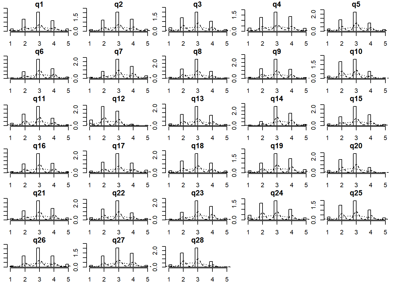
Every item has 5 response options, and things look more or less normal (hard to see with Likert data, but we’re not too skewed with lots of responses of 1s or 5s)

multi.hist(copeitems)

fa(..........., cor = "cor", rotate = ???, fm = ???)

what factor extraction method?
we have a fairly large sample size here (620), and everything looks fairly normally distributed. I think “ml” is a safe bet here. We probably won’t get very different results depending on our choice in this situation, so any are probably fine.

fa(..........., cor = "cor", rotate = ???, fm = "ml")

what rotation?

• We’re trying to measure “coping strategies”. There are lots of possible links between questions I can see - some of the questions seem to ask about social related strategies (q5, q10), some seem to be distraction-focussed (q1, q19). Some seem like bad strategies (drugs, denial, self criticism), and some seem like better ones (planning, social support etc).
  • if it is a unidimensional scale, what would that represent? It will depend on the loadings (e.g., if loadings are positive for social items and negative for drugs/denial etc., then I suppose being higher indicates ’more frequently doing better coping strategies). But if all the loadings are positive, it would just represent “engaging more with coping strategies (of any sort)”
• If the measure is multi-dimensional (i.e., if there is more than just one latent factor that explains peoples’ responses to these questions), then would we expect those dimensions to be related? Probably! E.g., we would expect that someone who frequently uses the ‘good’ coping strategies will be less often using the ‘bad’ ones?
• And also, why would we ever want to constrain any dimensions to be orthogonal? Very occasionally, we might TODO, but not here

fa(..........., cor = "cor", rotate = "oblimin", fm = "ml")

Question 3

Define a range for the number of factors that we will extract.

🗂️ See the How to: Decide on the Number of Components/Factors flash card.

Solution 3.

method	suggestion
scree plot	maybe 3? or maybe 6?
parallel analysis	6
MAP	3

Let’s examine from 3 to 6 factors.

scree(copeitems)

fa.parallel(copeitems)

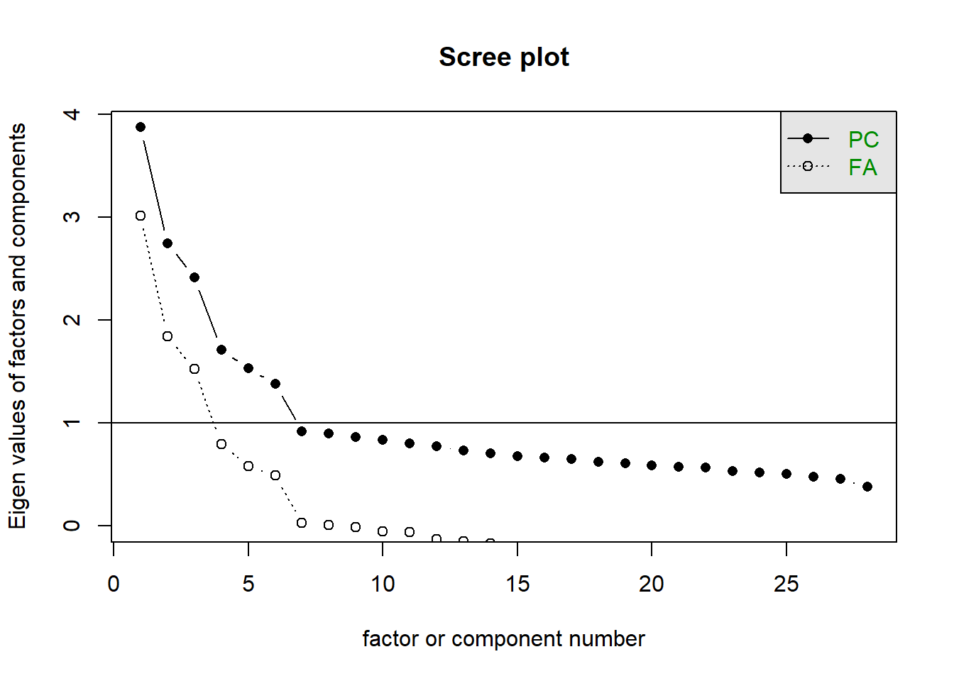
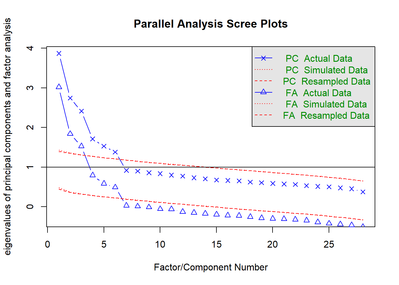
Parallel analysis suggests that the number of factors =  6  and the number of components =  6 

VSS(copeitems, plot=F)

Very Simple Structure
Call: vss(x = x, n = n, rotate = rotate, diagonal = diagonal, fm = fm, 
    n.obs = n.obs, plot = plot, title = title, use = use, cor = cor)
VSS complexity 1 achieves a maximimum of 0.54  with  3  factors
VSS complexity 2 achieves a maximimum of 0.66  with  8  factors

The Velicer MAP achieves a minimum of 0.01  with  3  factors 
BIC achieves a minimum of  -1148  with  6  factors
Sample Size adjusted BIC achieves a minimum of  -442  with  7  factors

Statistics by number of factors 
  vss1 vss2   map dof chisq     prob sqresid  fit RMSEA   BIC SABIC complex
1 0.31 0.00 0.017 350  2244 4.1e-273      31 0.31 0.093    -6  1105     1.0
2 0.38 0.47 0.014 323  1577 5.8e-164      24 0.47 0.079  -499   526     1.4
3 0.48 0.58 0.010 297   953  7.0e-70      19 0.59 0.060  -956   -13     1.4
4 0.48 0.60 0.011 272   706  2.9e-40      16 0.64 0.051 -1043  -180     1.5
5 0.50 0.63 0.012 248   479  7.6e-17      14 0.69 0.039 -1116  -328     1.6
6 0.54 0.65 0.013 225   299  6.8e-04      12 0.73 0.023 -1148  -433     1.5
7 0.52 0.66 0.015 203   219  2.1e-01      12 0.74 0.011 -1086  -442     1.6
8 0.50 0.66 0.017 182   177  5.9e-01      11 0.75 0.000  -993  -415     1.7
  eChisq  SRMR eCRMS  eBIC
1   5385 0.107 0.111  3135
2   3139 0.082 0.089  1062
3   1461 0.056 0.063  -448
4    947 0.045 0.053  -801
5    542 0.034 0.042 -1053
6    255 0.023 0.030 -1192
7    188 0.020 0.027 -1117
8    146 0.018 0.025 -1024

Question 4

For every number in your range, fit a factor model.

🗂️ See the Fitting and Comparing EFA solutions flash card.

Solution 4.

copefa3 <- fa(copeitems, nfactors = 3, rotate = "oblimin", fm = "ml", cor = "cor")
copefa4 <- fa(copeitems, nfactors = 4, rotate = "oblimin", fm = "ml", cor = "cor")
copefa5 <- fa(copeitems, nfactors = 5, rotate = "oblimin", fm = "ml", cor = "cor")
copefa6 <- fa(copeitems, nfactors = 6, rotate = "oblimin", fm = "ml", cor = "cor")

Question 5

V - variance

How much of the total variance in the coping strategy items is explained by each factor solution?

Solution 5.

solution	variance explained
3 factor	0.24
4 factor	0.27
5 factor	0.31
6 factor	0.34

Question 6

I - identification

For each solution, do all factors have 3+ items for which the factor is the primary loading?

Solution 6.

solution	all factors identified
3 factor	yes
4 factor	yes
5 factor	one factor (ML4) has only 2 items
6 factor	two factors (ML4, ML6) only have 2 items

Question 7

S - salience, C - complexity, H - heywood cases

Look at the patterns of loadings for each solution. Are there any items that:

• do not load on to any factor at a salient level?
• have high complexity or cross loadings across multiple factors?
• have impossible values (factor loadings or communalities > 1)?

Solution 7.

Full output

3 factor

copefa3

Factor Analysis using method =  ml
Call: fa(r = copeitems, nfactors = 3, rotate = "oblimin", fm = "ml", 
    cor = "cor")
Standardized loadings (pattern matrix) based upon correlation matrix
      ML1   ML2   ML3    h2   u2 com
q1  -0.14  0.48  0.22 0.284 0.72 1.6
q2   0.38  0.00 -0.07 0.144 0.86 1.1
q3   0.17  0.05  0.39 0.205 0.80 1.4
q4  -0.12 -0.02  0.14 0.030 0.97 2.0
q5   0.53 -0.04  0.03 0.277 0.72 1.0
q6  -0.10  0.05  0.61 0.373 0.63 1.1
q7   0.42  0.21 -0.11 0.244 0.76 1.6
q8   0.09 -0.07  0.49 0.258 0.74 1.1
q9   0.22  0.04  0.41 0.252 0.75 1.6
q10  0.65 -0.11  0.06 0.429 0.57 1.1
q11 -0.07 -0.07  0.19 0.044 0.96 1.6
q12  0.05  0.63 -0.02 0.407 0.59 1.0
q13  0.00  0.12  0.54 0.319 0.68 1.1
q14  0.35  0.22  0.00 0.191 0.81 1.7
q15  0.57 -0.03  0.02 0.327 0.67 1.0
q16  0.02 -0.02  0.59 0.350 0.65 1.0
q17  0.23  0.43 -0.13 0.268 0.73 1.7
q18 -0.03  0.52  0.09 0.282 0.72 1.1
q19 -0.06  0.46  0.13 0.229 0.77 1.2
q20 -0.01  0.33 -0.22 0.150 0.85 1.8
q21  0.37  0.13  0.18 0.218 0.78 1.7
q22  0.20  0.00 -0.03 0.039 0.96 1.1
q23  0.51 -0.09  0.12 0.281 0.72 1.2
q24  0.16  0.42 -0.11 0.220 0.78 1.4
q25  0.48  0.27 -0.06 0.326 0.67 1.6
q26  0.07 -0.06  0.54 0.302 0.70 1.1
q27  0.13  0.11  0.04 0.035 0.97 2.1
q28 -0.07  0.64  0.01 0.406 0.59 1.0

                       ML1  ML2  ML3
SS loadings           2.43 2.28 2.17
Proportion Var        0.09 0.08 0.08
Cumulative Var        0.09 0.17 0.25
Proportion Explained  0.35 0.33 0.32
Cumulative Proportion 0.35 0.68 1.00

 With factor correlations of 
     ML1  ML2  ML3
ML1 1.00 0.13 0.13
ML2 0.13 1.00 0.06
ML3 0.13 0.06 1.00

Mean item complexity =  1.4
Test of the hypothesis that 3 factors are sufficient.

df null model =  378  with the objective function =  5.44 with Chi Square =  3314
df of  the model are 297  and the objective function was  1.57 

The root mean square of the residuals (RMSR) is  0.06 
The df corrected root mean square of the residuals is  0.06 

The harmonic n.obs is  620 with the empirical chi square  1472  with prob <  8.8e-155 
The total n.obs was  620  with Likelihood Chi Square =  950  with prob <  2e-69 

Tucker Lewis Index of factoring reliability =  0.716
RMSEA index =  0.06  and the 90 % confidence intervals are  0.055 0.064
BIC =  -959
Fit based upon off diagonal values = 0.86
Measures of factor score adequacy             
                                                   ML1  ML2  ML3
Correlation of (regression) scores with factors   0.88 0.88 0.87
Multiple R square of scores with factors          0.77 0.77 0.76
Minimum correlation of possible factor scores     0.55 0.54 0.51

4 factor

copefa4

Factor Analysis using method =  ml
Call: fa(r = copeitems, nfactors = 4, rotate = "oblimin", fm = "ml", 
    cor = "cor")
Standardized loadings (pattern matrix) based upon correlation matrix
      ML3   ML2   ML1   ML4    h2   u2 com
q1   0.18  0.52 -0.04 -0.11 0.306 0.69 1.3
q2  -0.03 -0.08  0.19  0.34 0.177 0.82 1.7
q3   0.47 -0.05 -0.05  0.33 0.322 0.68 1.8
q4   0.11  0.04  0.02 -0.21 0.052 0.95 1.6
q5  -0.03  0.01  0.65 -0.07 0.401 0.60 1.0
q6   0.60  0.08 -0.05 -0.09 0.367 0.63 1.1
q7  -0.05  0.06  0.08  0.59 0.397 0.60 1.1
q8   0.55 -0.12 -0.05  0.19 0.336 0.66 1.4
q9   0.39  0.07  0.27 -0.03 0.261 0.74 1.9
q10  0.03 -0.11  0.62  0.13 0.446 0.55 1.2
q11  0.17 -0.02  0.05 -0.19 0.064 0.94 2.1
q12 -0.01  0.57 -0.05  0.21 0.403 0.60 1.3
q13  0.52  0.16  0.07 -0.07 0.315 0.69 1.3
q14  0.06  0.09  0.07  0.49 0.292 0.71 1.1
q15 -0.02 -0.01  0.62  0.03 0.390 0.61 1.0
q16  0.58  0.01  0.07 -0.08 0.348 0.65 1.1
q17 -0.10  0.34  0.04  0.34 0.287 0.71 2.2
q18  0.09  0.48 -0.09  0.14 0.283 0.72 1.3
q19  0.10  0.48 -0.01 -0.04 0.241 0.76 1.1
q20 -0.28  0.39  0.11 -0.13 0.220 0.78 2.3
q21  0.14  0.18  0.45 -0.04 0.270 0.73 1.5
q22  0.01 -0.08  0.03  0.25 0.070 0.93 1.2
q23  0.10 -0.09  0.47  0.10 0.283 0.72 1.3
q24 -0.13  0.41  0.15  0.09 0.231 0.77 1.6
q25 -0.03  0.18  0.27  0.40 0.347 0.65 2.2
q26  0.52 -0.02  0.11 -0.06 0.297 0.70 1.1
q27  0.08  0.02 -0.05  0.27 0.080 0.92 1.3
q28 -0.01  0.66 -0.02 -0.02 0.430 0.57 1.0

                       ML3  ML2  ML1  ML4
SS loadings           2.18 2.15 1.98 1.61
Proportion Var        0.08 0.08 0.07 0.06
Cumulative Var        0.08 0.15 0.23 0.28
Proportion Explained  0.28 0.27 0.25 0.20
Cumulative Proportion 0.28 0.55 0.80 1.00

 With factor correlations of 
     ML3  ML2  ML1  ML4
ML3 1.00 0.06 0.14 0.05
ML2 0.06 1.00 0.08 0.16
ML1 0.14 0.08 1.00 0.28
ML4 0.05 0.16 0.28 1.00

Mean item complexity =  1.4
Test of the hypothesis that 4 factors are sufficient.

df null model =  378  with the objective function =  5.44 with Chi Square =  3314
df of  the model are 272  and the objective function was  1.15 

The root mean square of the residuals (RMSR) is  0.05 
The df corrected root mean square of the residuals is  0.05 

The harmonic n.obs is  620 with the empirical chi square  973  with prob <  1.5e-79 
The total n.obs was  620  with Likelihood Chi Square =  695  with prob <  7.3e-39 

Tucker Lewis Index of factoring reliability =  0.799
RMSEA index =  0.05  and the 90 % confidence intervals are  0.046 0.055
BIC =  -1054
Fit based upon off diagonal values = 0.91
Measures of factor score adequacy             
                                                   ML3  ML2  ML1  ML4
Correlation of (regression) scores with factors   0.87 0.87 0.87 0.83
Multiple R square of scores with factors          0.76 0.76 0.75 0.69
Minimum correlation of possible factor scores     0.52 0.52 0.51 0.38

5 factor

copefa5

Factor Analysis using method =  ml
Call: fa(r = copeitems, nfactors = 5, rotate = "oblimin", fm = "ml", 
    cor = "cor")
Standardized loadings (pattern matrix) based upon correlation matrix
      ML3   ML2   ML1   ML5   ML4    h2   u2 com
q1   0.52  0.22 -0.03 -0.18 -0.10 0.346 0.65 1.7
q2  -0.05 -0.10  0.19  0.44  0.20 0.291 0.71 2.0
q3  -0.02  0.44 -0.04  0.37  0.03 0.332 0.67 2.0
q4   0.06 -0.01 -0.01 -0.02  0.67 0.454 0.55 1.0
q5   0.01 -0.03  0.65 -0.07  0.05 0.394 0.61 1.0
q6   0.06  0.61 -0.04 -0.08 -0.01 0.378 0.62 1.1
q7   0.12 -0.06  0.12  0.54 -0.09 0.380 0.62 1.3
q8  -0.11  0.51 -0.05  0.27  0.12 0.362 0.64 1.8
q9   0.07  0.38  0.26 -0.01  0.08 0.259 0.74 2.0
q10 -0.10  0.05  0.64  0.08 -0.08 0.455 0.54 1.1
q11 -0.01  0.06  0.03 -0.01  0.64 0.422 0.58 1.0
q12  0.60 -0.03 -0.04  0.20  0.03 0.415 0.58 1.2
q13  0.15  0.53  0.07 -0.08  0.01 0.322 0.68 1.2
q14  0.13  0.08  0.10  0.41 -0.21 0.299 0.70 1.9
q15  0.00 -0.03  0.62  0.04  0.05 0.389 0.61 1.0
q16  0.00  0.57  0.07 -0.05  0.05 0.345 0.65 1.1
q17  0.37 -0.08  0.06  0.27 -0.16 0.290 0.71 2.4
q18  0.51  0.07 -0.09  0.16  0.12 0.313 0.69 1.4
q19  0.47  0.13  0.00 -0.09 -0.07 0.253 0.75 1.3
q20  0.38 -0.27  0.11 -0.15  0.03 0.218 0.78 2.4
q21  0.17  0.14  0.45 -0.04  0.04 0.270 0.73 1.5
q22 -0.06  0.02  0.04  0.23 -0.13 0.078 0.92 1.9
q23 -0.09  0.11  0.48  0.08 -0.05 0.285 0.71 1.3
q24  0.42 -0.12  0.16  0.04 -0.01 0.230 0.77 1.5
q25  0.21 -0.03  0.29  0.34 -0.10 0.344 0.66 2.9
q26 -0.04  0.54  0.12 -0.08 -0.06 0.319 0.68 1.2
q27  0.04  0.09 -0.04  0.26 -0.10 0.086 0.91 1.7
q28  0.66 -0.02 -0.02 -0.03  0.06 0.427 0.57 1.0

                       ML3  ML2  ML1  ML5  ML4
SS loadings           2.22 2.14 2.04 1.44 1.12
Proportion Var        0.08 0.08 0.07 0.05 0.04
Cumulative Var        0.08 0.16 0.23 0.28 0.32
Proportion Explained  0.25 0.24 0.23 0.16 0.12
Cumulative Proportion 0.25 0.49 0.71 0.88 1.00

 With factor correlations of 
      ML3  ML2   ML1   ML5   ML4
ML3  1.00 0.06  0.09  0.12 -0.06
ML2  0.06 1.00  0.13  0.05  0.10
ML1  0.09 0.13  1.00  0.27 -0.05
ML5  0.12 0.05  0.27  1.00 -0.05
ML4 -0.06 0.10 -0.05 -0.05  1.00

Mean item complexity =  1.5
Test of the hypothesis that 5 factors are sufficient.

df null model =  378  with the objective function =  5.44 with Chi Square =  3314
df of  the model are 248  and the objective function was  0.78 

The root mean square of the residuals (RMSR) is  0.03 
The df corrected root mean square of the residuals is  0.04 

The harmonic n.obs is  620 with the empirical chi square  555  with prob <  1.6e-25 
The total n.obs was  620  with Likelihood Chi Square =  474  with prob <  2.8e-16 

Tucker Lewis Index of factoring reliability =  0.882
RMSEA index =  0.038  and the 90 % confidence intervals are  0.033 0.044
BIC =  -1121
Fit based upon off diagonal values = 0.95
Measures of factor score adequacy             
                                                   ML3  ML2  ML1  ML5  ML4
Correlation of (regression) scores with factors   0.88 0.87 0.87 0.82 0.81
Multiple R square of scores with factors          0.77 0.76 0.76 0.67 0.65
Minimum correlation of possible factor scores     0.54 0.52 0.52 0.34 0.31

6 factor

copefa6

Factor Analysis using method =  ml
Call: fa(r = copeitems, nfactors = 6, rotate = "oblimin", fm = "ml", 
    cor = "cor")
Standardized loadings (pattern matrix) based upon correlation matrix
      ML3   ML2   ML1   ML5   ML4   ML6   h2   u2 com
q1   0.50  0.24 -0.04 -0.09 -0.13 -0.14 0.35 0.65 1.8
q2  -0.08 -0.09  0.14  0.43  0.24  0.06 0.29 0.71 2.1
q3  -0.04  0.43 -0.06  0.30  0.08  0.15 0.32 0.68 2.2
q4   0.06 -0.01  0.00 -0.04  0.66 -0.08 0.45 0.55 1.1
q5   0.03 -0.04  0.67 -0.08  0.04  0.04 0.42 0.58 1.1
q6   0.06  0.61 -0.04 -0.08 -0.02  0.00 0.38 0.62 1.1
q7   0.04 -0.04  0.01  0.67 -0.04 -0.02 0.46 0.54 1.0
q8  -0.11  0.50 -0.05  0.16  0.15  0.19 0.36 0.64 1.9
q9   0.08  0.37  0.28 -0.06  0.08  0.09 0.27 0.73 2.3
q10 -0.12  0.06  0.60  0.16 -0.08 -0.03 0.45 0.55 1.3
q11  0.00  0.06  0.03 -0.04  0.63 -0.04 0.41 0.59 1.0
q12  0.62 -0.04 -0.03  0.11  0.06  0.18 0.45 0.55 1.3
q13  0.12  0.55  0.04  0.02  0.00 -0.15 0.35 0.65 1.3
q14  0.07  0.10  0.01  0.53 -0.17 -0.04 0.35 0.65 1.3
q15  0.01 -0.03  0.62  0.03  0.05  0.05 0.40 0.60 1.0
q16  0.01  0.56  0.08 -0.09  0.05  0.05 0.35 0.65 1.1
q17  0.38 -0.10  0.06  0.20 -0.13  0.21 0.31 0.69 2.7
q18  0.50  0.06 -0.09  0.12  0.13  0.09 0.31 0.69 1.5
q19  0.47  0.13  0.01 -0.07 -0.09 -0.01 0.25 0.75 1.3
q20  0.37 -0.25  0.10 -0.05  0.00 -0.17 0.22 0.78 2.5
q21  0.15  0.15  0.42  0.05  0.03 -0.13 0.28 0.72 1.8
q22  0.00 -0.03  0.11 -0.06 -0.11  0.57 0.35 0.65 1.2
q23 -0.08  0.10  0.48  0.05 -0.05  0.10 0.29 0.71 1.3
q24  0.40 -0.11  0.14  0.12 -0.02 -0.07 0.23 0.77 1.7
q25  0.16 -0.01  0.22  0.46 -0.07 -0.07 0.38 0.62 1.8
q26 -0.06  0.56  0.10 -0.01 -0.07 -0.10 0.33 0.67 1.2
q27  0.10  0.04  0.01 -0.03 -0.06  0.59 0.36 0.64 1.1
q28  0.66 -0.02 -0.01 -0.01  0.05 -0.03 0.43 0.57 1.0

                       ML3  ML2  ML1  ML5  ML4  ML6
SS loadings           2.16 2.15 1.92 1.53 1.08 0.98
Proportion Var        0.08 0.08 0.07 0.05 0.04 0.03
Cumulative Var        0.08 0.15 0.22 0.28 0.32 0.35
Proportion Explained  0.22 0.22 0.20 0.16 0.11 0.10
Cumulative Proportion 0.22 0.44 0.63 0.79 0.90 1.00

 With factor correlations of 
      ML3  ML2   ML1   ML5   ML4   ML6
ML3  1.00 0.07  0.06  0.18 -0.05  0.00
ML2  0.07 1.00  0.13  0.05  0.10  0.05
ML1  0.06 0.13  1.00  0.31 -0.02  0.08
ML5  0.18 0.05  0.31  1.00 -0.08  0.20
ML4 -0.05 0.10 -0.02 -0.08  1.00 -0.01
ML6  0.00 0.05  0.08  0.20 -0.01  1.00

Mean item complexity =  1.5
Test of the hypothesis that 6 factors are sufficient.

df null model =  378  with the objective function =  5.44 with Chi Square =  3314
df of  the model are 225  and the objective function was  0.49 

The root mean square of the residuals (RMSR) is  0.02 
The df corrected root mean square of the residuals is  0.03 

The harmonic n.obs is  620 with the empirical chi square  259  with prob <  0.062 
The total n.obs was  620  with Likelihood Chi Square =  298  with prob <  0.00082 

Tucker Lewis Index of factoring reliability =  0.958
RMSEA index =  0.023  and the 90 % confidence intervals are  0.015 0.03
BIC =  -1149
Fit based upon off diagonal values = 0.98
Measures of factor score adequacy             
                                                   ML3  ML2  ML1  ML5  ML4  ML6
Correlation of (regression) scores with factors   0.88 0.87 0.87 0.84 0.80 0.77
Multiple R square of scores with factors          0.77 0.76 0.75 0.71 0.65 0.60
Minimum correlation of possible factor scores     0.54 0.53 0.51 0.42 0.30 0.20

Tidied loadings

3 factor

print(copefa3$loadings, cutoff = .3, sort = T)

Loadings:
    ML1    ML2    ML3   
q5   0.525              
q10  0.650              
q15  0.572              
q23  0.507              
q12         0.632       
q18         0.522       
q28         0.642       
q6                 0.611
q13                0.544
q16                0.590
q26                0.537
q1          0.478       
q2   0.382              
q3                 0.392
q4                      
q7   0.423              
q8                 0.489
q9                 0.415
q11                     
q14  0.351              
q17         0.434       
q19         0.458       
q20         0.331       
q21  0.368              
q22                     
q24         0.420       
q25  0.477              
q27                     

                 ML1   ML2   ML3
SS loadings    2.381 2.247 2.151
Proportion Var 0.085 0.080 0.077
Cumulative Var 0.085 0.165 0.242

4 factor

print(copefa4$loadings, cutoff = .3, sort = T)

Loadings:
    ML3    ML2    ML1    ML4   
q6   0.599                     
q8   0.547                     
q13  0.519                     
q16  0.576                     
q26  0.522                     
q1          0.522              
q12         0.575              
q28         0.660              
q5                 0.652       
q10                0.615       
q15                0.617       
q7                        0.590
q2                        0.336
q3   0.466                0.328
q4                             
q9   0.394                     
q11                            
q14                       0.487
q17         0.342         0.345
q18         0.483              
q19         0.480              
q20         0.387              
q21                0.446       
q22                            
q23                0.474       
q24         0.411              
q25                       0.397
q27                            

                 ML3   ML2   ML1   ML4
SS loadings    2.147 2.103 1.878 1.499
Proportion Var 0.077 0.075 0.067 0.054
Cumulative Var 0.077 0.152 0.219 0.272

5 factor

print(copefa5$loadings, cutoff = .3, sort = T)

Loadings:
    ML3    ML2    ML1    ML5    ML4   
q1   0.516                            
q12  0.599                            
q18  0.510                            
q28  0.659                            
q6          0.611                     
q8          0.514                     
q13         0.527                     
q16         0.569                     
q26         0.545                     
q5                 0.645              
q10                0.636              
q15                0.617              
q7                        0.536       
q4                               0.674
q11                              0.641
q2                        0.436       
q3          0.440         0.365       
q9          0.381                     
q14                       0.411       
q17  0.374                            
q19  0.474                            
q20  0.379                            
q21                0.448              
q22                                   
q23                0.481              
q24  0.423                            
q25                       0.341       
q27                                   

                 ML3   ML2   ML1   ML5   ML4
SS loadings    2.185 2.106 1.930 1.332 1.100
Proportion Var 0.078 0.075 0.069 0.048 0.039
Cumulative Var 0.078 0.153 0.222 0.270 0.309

6 factor

print(copefa6$loadings, cutoff = .3, sort = T)

Loadings:
    ML3    ML2    ML1    ML5    ML4    ML6   
q1   0.503                                   
q12  0.617                                   
q18  0.502                                   
q28  0.661                                   
q6          0.611                            
q13         0.550                            
q16         0.562                            
q26         0.559                            
q5                 0.669                     
q10                0.595                     
q15                0.616                     
q7                        0.668              
q14                       0.529              
q4                               0.664       
q11                              0.628       
q22                                     0.571
q27                                     0.588
q2                        0.430              
q3          0.429                            
q8          0.500                            
q9          0.374                            
q17  0.376                                   
q19  0.473                                   
q20  0.366                                   
q21                0.422                     
q23                0.480                     
q24  0.401                                   
q25                       0.464              

                 ML3   ML2   ML1   ML5   ML4   ML6
SS loadings    2.121 2.109 1.817 1.401 1.068 0.960
Proportion Var 0.076 0.075 0.065 0.050 0.038 0.034
Cumulative Var 0.076 0.151 0.216 0.266 0.304 0.338

solution	salience of items	complexity & cross loadings	heywood cases
3 factor	4 items (11,22,27,4) have no salient loadings	no cross loadings, but higher complexity for qs 21, 14	no
4 factor	4 items (11,22,27,4) have no salient loadings	cross loadings for qs 17 and 3	no
5 factor	2 items (22,27) have no salient loadings	cross loadings for q3	no
6 factor	no	no cross loadings but high complexity for many items (2,3,8,9,17,20,21,24,25)	no

Question 8

Given your examination so far, some items may be flagged as consistently problematic.
Here are the ones we identified.

• q4, q11, q22 and q27 were only salient when loading onto factors with <3 items (11 and 4 seemed to go together, as did 22 and 27).
  
• q3 has some cross loadings in several solutions.

Take a look at the wordings of any such items. Are they “double barrelled” or ambiguously worded? Can you think of any theoretical reason why these items are causing problems?

Normally, we would want to remove items one at a time. This is a time-consuming process, so let’s skip ahead, and suppose we need to remove all four of q4, q11, q22 and q27.
Task: create a new dataframe which is the subset of items without questions 4, 11, 22, and 27.

Solution 8.

copeitems_sub <- copeitems |>
  select(-q4, -q11, -q22, -q27)

Solution 9. We’ve just got rid of some items. Surely that means that we’re losing someting important that we measured?

This depends on why we have decided to discard those items. If they were badly worded, then we could argue that they just contain too much noise, or that the ‘signal’ they carry is unable to be clearly separated out into any of the latent factors (i.e. “I use alcohol or drugs to relax and then feel guilty about it later.” would be split across two types of coping strategy: use of alcohol and self-blame).

In our case, I think we can argue for something else happening. If you look at the items we have discarded, they seem fairly clear. Qs 4 and 11 are about substance misuse, and Qs 22 and 27 about spiritual/religious coping.

variable	wording
q4	I've been using alcohol or other drugs to make myself feel better.
q11	I've been using alcohol or other drugs to help me get through it.
q22	I've been trying to find comfort in my religion or spiritual beliefs.
q27	I've been praying or meditating.

Note that also in the factor solutions we have looked at that have more factors, these pairs came out as their own little factors with 2 items each. So there is potentially a real construct there, it’s simply that the 2-item factors are statistically unstable.
So while these don’t fit in to our general view of measuring “coping strategies”, we might want to consider either:

1. refining our questionnaire, adding more items about these, and starting over.
2. start thinking of religiosity and substance use as separate from ‘coping strategies’, and include them as separate measures in analyses that study coping.

Question 9

Re-do the entire process!

We’ve printed all the output so that you don’t have to code it right here and now, and can focus on the evaluation of the different solutions.

Are any of these models satisfactory? Do you think they need further refinement? Remember to take into consideration the wordings of the items!

Solution 10.

cor(copeitems_sub) |>
  heatmap()

bartlett.test(copeitems_sub)

    Bartlett test of homogeneity of variances

data:  copeitems_sub
Bartlett's K-squared = 183, df = 23, p-value <2e-16

KMO(copeitems_sub)

Kaiser-Meyer-Olkin factor adequacy
Call: KMO(r = copeitems_sub)
Overall MSA =  0.81
MSA for each item = 
  q1   q2   q3   q5   q6   q7   q8   q9  q10  q12  q13  q14  q15  q16  q17  q18 
0.80 0.79 0.83 0.78 0.80 0.77 0.82 0.86 0.81 0.73 0.82 0.81 0.82 0.84 0.86 0.85 
 q19  q20  q21  q23  q24  q25  q26  q28 
0.84 0.79 0.87 0.86 0.84 0.85 0.81 0.75 

Solution 11.

method	suggestion
scree plot	1? maybe 2? 4?
parallel analysis	4
MAP	3

scree(copeitems_sub)

fa.parallel(copeitems_sub)

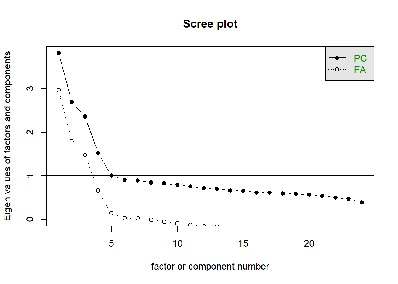
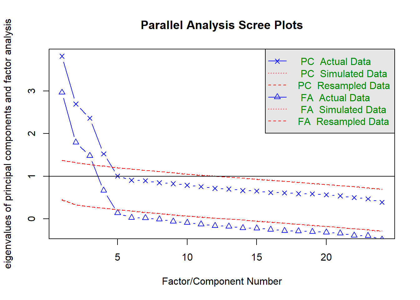
Parallel analysis suggests that the number of factors =  4  and the number of components =  4 

VSS(copeitems_sub, plot=F)

Very Simple Structure
Call: vss(x = x, n = n, rotate = rotate, diagonal = diagonal, fm = fm, 
    n.obs = n.obs, plot = plot, title = title, use = use, cor = cor)
VSS complexity 1 achieves a maximimum of 0.54  with  3  factors
VSS complexity 2 achieves a maximimum of 0.68  with  5  factors

The Velicer MAP achieves a minimum of 0.01  with  3  factors 
BIC achieves a minimum of  -910  with  4  factors
Sample Size adjusted BIC achieves a minimum of  -349  with  5  factors

Statistics by number of factors 
  vss1 vss2   map dof chisq     prob sqresid  fit  RMSEA  BIC SABIC complex
1 0.35 0.00 0.020 252  1783 2.0e-228    25.6 0.35 0.0990  163   963     1.0
2 0.45 0.52 0.016 229  1136 4.2e-120    18.9 0.52 0.0799 -336   391     1.3
3 0.54 0.64 0.011 207   522  4.4e-29    13.6 0.66 0.0495 -809  -152     1.3
4 0.54 0.67 0.011 186   286  3.7e-06    11.6 0.71 0.0293 -910  -320     1.4
5 0.51 0.68 0.014 166   191  8.9e-02    10.8 0.73 0.0155 -876  -349     1.5
6 0.52 0.67 0.017 147   149  4.3e-01    10.3 0.74 0.0048 -796  -329     1.6
7 0.51 0.66 0.020 129   116  7.9e-01     9.8 0.75 0.0000 -714  -304     1.7
8 0.51 0.66 0.024 112    92  9.2e-01     9.4 0.76 0.0000 -629  -273     1.8
  eChisq  SRMR eCRMS eBIC
1   4406 0.113 0.119 2786
2   2269 0.081 0.089  797
3    673 0.044 0.051 -658
4    265 0.028 0.034 -931
5    173 0.023 0.029 -894
6    133 0.020 0.027 -812
7    100 0.017 0.025 -730
8     75 0.015 0.023 -645

Let’s examine from 1 to 4 factors.

Solution 12.

copefa1s <- fa(copeitems_sub, nfactors = 1, fm = "ml", cor = "cor")
copefa2s <- fa(copeitems_sub, nfactors = 2, rotate = "oblimin", fm = "ml", cor = "cor")
copefa3s <- fa(copeitems_sub, nfactors = 3, rotate = "oblimin", fm = "ml", cor = "cor")
copefa4s <- fa(copeitems_sub, nfactors = 4, rotate = "oblimin", fm = "ml", cor = "cor")

Full output

1 factor

copefa1s

Factor Analysis using method =  ml
Call: fa(r = copeitems_sub, nfactors = 1, fm = "ml", cor = "cor")
Standardized loadings (pattern matrix) based upon correlation matrix
     ML1     h2   u2 com
q1  0.24 0.0583 0.94   1
q2  0.30 0.0884 0.91   1
q3  0.34 0.1158 0.88   1
q5  0.41 0.1651 0.83   1
q6  0.21 0.0462 0.95   1
q7  0.42 0.1805 0.82   1
q8  0.25 0.0636 0.94   1
q9  0.39 0.1493 0.85   1
q10 0.48 0.2258 0.77   1
q12 0.35 0.1213 0.88   1
q13 0.31 0.0984 0.90   1
q14 0.42 0.1801 0.82   1
q15 0.45 0.1983 0.80   1
q16 0.26 0.0651 0.93   1
q17 0.35 0.1227 0.88   1
q18 0.30 0.0907 0.91   1
q19 0.25 0.0645 0.94   1
q20 0.08 0.0065 0.99   1
q21 0.47 0.2247 0.78   1
q23 0.40 0.1640 0.84   1
q24 0.32 0.0997 0.90   1
q25 0.53 0.2760 0.72   1
q26 0.27 0.0722 0.93   1
q28 0.28 0.0812 0.92   1

                ML1
SS loadings    2.96
Proportion Var 0.12

Mean item complexity =  1
Test of the hypothesis that 1 factor is sufficient.

df null model =  276  with the objective function =  4.64 with Chi Square =  2829
df of  the model are 252  and the objective function was  2.92 

The root mean square of the residuals (RMSR) is  0.11 
The df corrected root mean square of the residuals is  0.12 

The harmonic n.obs is  620 with the empirical chi square  4425  with prob <  0 
The total n.obs was  620  with Likelihood Chi Square =  1781  with prob <  5.9e-228 

Tucker Lewis Index of factoring reliability =  0.343
RMSEA index =  0.099  and the 90 % confidence intervals are  0.095 0.103
BIC =  161
Fit based upon off diagonal values = 0.54
Measures of factor score adequacy             
                                                   ML1
Correlation of (regression) scores with factors   0.88
Multiple R square of scores with factors          0.78
Minimum correlation of possible factor scores     0.56

2 factor

copefa2s

Factor Analysis using method =  ml
Call: fa(r = copeitems_sub, nfactors = 2, rotate = "oblimin", fm = "ml", 
    cor = "cor")
Standardized loadings (pattern matrix) based upon correlation matrix
      ML1   ML2    h2   u2 com
q1   0.31  0.08 0.111 0.89 1.1
q2   0.23  0.10 0.066 0.93 1.4
q3   0.08  0.45 0.216 0.78 1.1
q5   0.23  0.24 0.121 0.88 2.0
q6  -0.07  0.50 0.246 0.75 1.0
q7   0.42  0.08 0.193 0.81 1.1
q8  -0.07  0.51 0.258 0.74 1.0
q9   0.10  0.48 0.252 0.75 1.1
q10  0.23  0.32 0.171 0.83 1.8
q12  0.56 -0.06 0.308 0.69 1.0
q13  0.05  0.48 0.240 0.76 1.0
q14  0.38  0.15 0.177 0.82 1.3
q15  0.26  0.25 0.145 0.86 2.0
q16 -0.08  0.55 0.296 0.70 1.0
q17  0.51 -0.07 0.262 0.74 1.0
q18  0.44  0.01 0.191 0.81 1.0
q19  0.35  0.04 0.125 0.87 1.0
q20  0.33 -0.26 0.159 0.84 1.9
q21  0.30  0.31 0.204 0.80 2.0
q23  0.16  0.33 0.146 0.85 1.5
q24  0.49 -0.09 0.238 0.76 1.1
q25  0.50  0.14 0.280 0.72 1.2
q26 -0.08  0.55 0.300 0.70 1.0
q28  0.50 -0.08 0.252 0.75 1.1

                       ML1  ML2
SS loadings           2.57 2.39
Proportion Var        0.11 0.10
Cumulative Var        0.11 0.21
Proportion Explained  0.52 0.48
Cumulative Proportion 0.52 1.00

 With factor correlations of 
     ML1  ML2
ML1 1.00 0.11
ML2 0.11 1.00

Mean item complexity =  1.3
Test of the hypothesis that 2 factors are sufficient.

df null model =  276  with the objective function =  4.64 with Chi Square =  2829
df of  the model are 229  and the objective function was  1.86 

The root mean square of the residuals (RMSR) is  0.08 
The df corrected root mean square of the residuals is  0.09 

The harmonic n.obs is  620 with the empirical chi square  2284  with prob <  0 
The total n.obs was  620  with Likelihood Chi Square =  1134  with prob <  9.8e-120 

Tucker Lewis Index of factoring reliability =  0.572
RMSEA index =  0.08  and the 90 % confidence intervals are  0.075 0.085
BIC =  -338
Fit based upon off diagonal values = 0.76
Measures of factor score adequacy             
                                                   ML1  ML2
Correlation of (regression) scores with factors   0.88 0.87
Multiple R square of scores with factors          0.77 0.76
Minimum correlation of possible factor scores     0.53 0.51

3 factor

copefa3s

Factor Analysis using method =  ml
Call: fa(r = copeitems_sub, nfactors = 3, rotate = "oblimin", fm = "ml", 
    cor = "cor")
Standardized loadings (pattern matrix) based upon correlation matrix
      ML1   ML2   ML3   h2   u2 com
q1  -0.14  0.48  0.23 0.29 0.71 1.6
q2   0.39  0.01 -0.09 0.15 0.85 1.1
q3   0.16  0.04  0.39 0.20 0.80 1.3
q5   0.54 -0.04  0.02 0.29 0.71 1.0
q6  -0.10  0.04  0.62 0.38 0.62 1.1
q7   0.41  0.21 -0.10 0.23 0.77 1.6
q8   0.09 -0.07  0.48 0.25 0.75 1.1
q9   0.22  0.04  0.41 0.25 0.75 1.6
q10  0.66 -0.11  0.05 0.44 0.56 1.1
q12  0.04  0.63 -0.03 0.40 0.60 1.0
q13  0.01  0.12  0.54 0.32 0.68 1.1
q14  0.34  0.22  0.02 0.18 0.82 1.7
q15  0.58 -0.03  0.01 0.34 0.66 1.0
q16  0.02 -0.03  0.59 0.35 0.65 1.0
q17  0.20  0.43 -0.12 0.25 0.75 1.6
q18 -0.03  0.52  0.07 0.28 0.72 1.0
q19 -0.07  0.45  0.13 0.23 0.77 1.2
q20  0.00  0.34 -0.23 0.16 0.84 1.8
q21  0.38  0.13  0.17 0.23 0.77 1.7
q23  0.50 -0.09  0.12 0.28 0.72 1.2
q24  0.16  0.42 -0.12 0.23 0.77 1.4
q25  0.47  0.27 -0.05 0.33 0.67 1.6
q26  0.08 -0.06  0.55 0.31 0.69 1.1
q28 -0.06  0.65  0.01 0.41 0.59 1.0

                       ML1  ML2  ML3
SS loadings           2.37 2.26 2.13
Proportion Var        0.10 0.09 0.09
Cumulative Var        0.10 0.19 0.28
Proportion Explained  0.35 0.33 0.31
Cumulative Proportion 0.35 0.69 1.00

 With factor correlations of 
     ML1  ML2  ML3
ML1 1.00 0.12 0.13
ML2 0.12 1.00 0.07
ML3 0.13 0.07 1.00

Mean item complexity =  1.3
Test of the hypothesis that 3 factors are sufficient.

df null model =  276  with the objective function =  4.64 with Chi Square =  2829
df of  the model are 207  and the objective function was  0.85 

The root mean square of the residuals (RMSR) is  0.04 
The df corrected root mean square of the residuals is  0.05 

The harmonic n.obs is  620 with the empirical chi square  680  with prob <  1.1e-51 
The total n.obs was  620  with Likelihood Chi Square =  520  with prob <  7.7e-29 

Tucker Lewis Index of factoring reliability =  0.836
RMSEA index =  0.049  and the 90 % confidence intervals are  0.044 0.055
BIC =  -811
Fit based upon off diagonal values = 0.93
Measures of factor score adequacy             
                                                   ML1  ML2  ML3
Correlation of (regression) scores with factors   0.88 0.88 0.87
Multiple R square of scores with factors          0.77 0.77 0.75
Minimum correlation of possible factor scores     0.54 0.53 0.51

4 factor

copefa4s

Factor Analysis using method =  ml
Call: fa(r = copeitems_sub, nfactors = 4, rotate = "oblimin", fm = "ml", 
    cor = "cor")
Standardized loadings (pattern matrix) based upon correlation matrix
      ML2   ML3   ML1   ML4   h2   u2 com
q1   0.52  0.19 -0.04 -0.11 0.31 0.69 1.4
q2  -0.10 -0.04  0.15  0.40 0.21 0.79 1.4
q3  -0.05  0.46 -0.06  0.33 0.31 0.69 1.9
q5   0.02 -0.03  0.67 -0.08 0.42 0.58 1.0
q6   0.08  0.61 -0.04 -0.10 0.38 0.62 1.1
q7   0.05 -0.04  0.03  0.67 0.47 0.53 1.0
q8  -0.12  0.53 -0.05  0.19 0.32 0.68 1.4
q9   0.07  0.39  0.27 -0.04 0.26 0.74 1.9
q10 -0.11  0.04  0.61  0.14 0.45 0.55 1.2
q12  0.58 -0.02 -0.04  0.17 0.40 0.60 1.2
q13  0.14  0.53  0.05 -0.04 0.32 0.68 1.2
q14  0.09  0.07  0.04  0.50 0.30 0.70 1.1
q15  0.00 -0.02  0.62  0.04 0.39 0.61 1.0
q16  0.01  0.57  0.08 -0.08 0.35 0.65 1.1
q17  0.36 -0.10  0.06  0.27 0.25 0.75 2.1
q18  0.48  0.08 -0.10  0.14 0.28 0.72 1.3
q19  0.48  0.10  0.01 -0.07 0.25 0.75 1.1
q20  0.38 -0.27  0.10 -0.10 0.21 0.79 2.1
q21  0.17  0.14  0.43  0.00 0.26 0.74 1.6
q23 -0.08  0.10  0.48  0.07 0.28 0.72 1.2
q24  0.41 -0.13  0.14  0.10 0.23 0.77 1.6
q25  0.17 -0.02  0.23  0.43 0.36 0.64 1.9
q26 -0.03  0.54  0.11 -0.05 0.31 0.69 1.1
q28  0.66 -0.02 -0.02 -0.01 0.43 0.57 1.0

                       ML2  ML3  ML1  ML4
SS loadings           2.14 2.14 1.93 1.52
Proportion Var        0.09 0.09 0.08 0.06
Cumulative Var        0.09 0.18 0.26 0.32
Proportion Explained  0.28 0.28 0.25 0.20
Cumulative Proportion 0.28 0.55 0.80 1.00

 With factor correlations of 
     ML2  ML3  ML1  ML4
ML2 1.00 0.07 0.07 0.17
ML3 0.07 1.00 0.14 0.05
ML1 0.07 0.14 1.00 0.30
ML4 0.17 0.05 0.30 1.00

Mean item complexity =  1.4
Test of the hypothesis that 4 factors are sufficient.

df null model =  276  with the objective function =  4.64 with Chi Square =  2829
df of  the model are 186  and the objective function was  0.47 

The root mean square of the residuals (RMSR) is  0.03 
The df corrected root mean square of the residuals is  0.03 

The harmonic n.obs is  620 with the empirical chi square  269  with prob <  6.5e-05 
The total n.obs was  620  with Likelihood Chi Square =  284  with prob <  4.8e-06 

Tucker Lewis Index of factoring reliability =  0.943
RMSEA index =  0.029  and the 90 % confidence intervals are  0.022 0.036
BIC =  -912
Fit based upon off diagonal values = 0.97
Measures of factor score adequacy             
                                                   ML2  ML3  ML1  ML4
Correlation of (regression) scores with factors   0.87 0.87 0.87 0.84
Multiple R square of scores with factors          0.76 0.76 0.75 0.70
Minimum correlation of possible factor scores     0.52 0.52 0.51 0.40

Tidied loadings

1 factor

print(copefa1s$loadings, cutoff = .3, sort = T)

Loadings:
    ML1  
q25 0.525
q1       
q2       
q3  0.340
q5  0.406
q6       
q7  0.425
q8       
q9  0.386
q10 0.475
q12 0.348
q13 0.314
q14 0.424
q15 0.445
q16      
q17 0.350
q18 0.301
q19      
q20      
q21 0.474
q23 0.405
q24 0.316
q26      
q28      

                 ML1
SS loadings    2.958
Proportion Var 0.123

2 factor

print(copefa2s$loadings, cutoff = .3, sort = T)

Loadings:
    ML1    ML2   
q12  0.558       
q17  0.515       
q28  0.504       
q8          0.511
q16         0.547
q26         0.551
q1   0.314       
q2               
q3          0.449
q5               
q6          0.499
q7   0.424       
q9          0.479
q10         0.322
q13         0.482
q14  0.377       
q15              
q18  0.437       
q19  0.348       
q20  0.330       
q21         0.308
q23         0.329
q24  0.489       
q25  0.496       

                 ML1   ML2
SS loadings    2.537 2.360
Proportion Var 0.106 0.098
Cumulative Var 0.106 0.204

3 factor

print(copefa3s$loadings, cutoff = .3, sort = T)

Loadings:
    ML1    ML2    ML3   
q5   0.536              
q10  0.656              
q15  0.582              
q23  0.502              
q12         0.632       
q18         0.520       
q28         0.645       
q6                 0.621
q13                0.545
q16                0.588
q26                0.547
q1          0.475       
q2   0.392              
q3                 0.394
q7   0.414              
q8                 0.482
q9                 0.408
q14  0.337              
q17         0.430       
q19         0.454       
q20         0.340       
q21  0.384              
q24         0.425       
q25  0.475              

                 ML1   ML2   ML3
SS loadings    2.315 2.232 2.102
Proportion Var 0.096 0.093 0.088
Cumulative Var 0.096 0.189 0.277

4 factor

print(copefa4s$loadings, cutoff = .3, sort = T)

Loadings:
    ML2    ML3    ML1    ML4   
q1   0.520                     
q12  0.583                     
q28  0.658                     
q6          0.607              
q8          0.531              
q13         0.527              
q16         0.575              
q26         0.535              
q5                 0.667       
q10                0.606       
q15                0.617       
q7                        0.667
q2                        0.398
q3          0.461         0.331
q9          0.390              
q14                       0.498
q17  0.360                     
q18  0.480                     
q19  0.485                     
q20  0.380                     
q21                0.425       
q23                0.482       
q24  0.412                     
q25                       0.434

                 ML2   ML3   ML1   ML4
SS loadings    2.099 2.107 1.829 1.403
Proportion Var 0.087 0.088 0.076 0.058
Cumulative Var 0.087 0.175 0.251 0.310

Question 10

For your chosen solution, name the factors!

Solution 13. I think we could probably make an argument for either the 3 factor solution or the 4 factor solution (although we might want to take a closer look at q3).

Personally I would probably choose the 3 factor solution, if nothing else then for parsimony.
If we choose the 3 factor, then we might name them something like:

ML1 - “support and solution seeking” ML2 - “distraction and reframing” ML3 - “maladaptive/avoidant”

If we were to choose 4, then it feels like the first factor of gets split up into two separate parts: social support focussed, and problem/planning focussed. In the factor correlations, we can see that these two correlate more than other factors do, suggesting a reasonable degree of overlap (which makes sense with how our 3-factor model looks too)!

ML2 = reframing/distraction ML3 = avoidant/maladaptive ML1 = social support seeking ML4 = active problem focused

Interestingly, this latter factor then loads on to the q3, which sound a bit more like denial (I’ve been saying to myself “this isn’t real.”), but you could see this as also an active/planned coping strategy (perhaps not a good one!) of getting through difficult situations.