Give it a clear name (for example, dapr3_lab07.Rmd).
In the first code chunk, load the packages you’ll need this week:
tidyverse
psych
Gambler’s Fallacies
Dataset: gamblers.csv
A researcher is interested in assessing if people who gamble will tend to lose more if they are more ‘impulsive’, and whether this might depend on whether they are gambling online or in a casino.
They recruited 482 participants (248 in a casino, and 234 on an online gambling site). Each participant filled out a 6 question measure of “impulsivity”, and then their total net gains (or losses) for the day were recorded (in £). All people were only playing the game BlackJack.
Our research question: is greater impulsivity associated with bigger losses when comparing online gamblers to casino gamblers?
whether the person was gambling in a casino or online
imp_1
I often act on the spur of the moment without thinking.
imp_2
I find it hard to resist temptations.
imp_3
I make decisions quickly, even when they have serious consequences.
imp_4
I find it hard to stay focused on tasks that take a long time to finish.
imp_5
I prefer safe activities rather than risky things just for fun.
imp_6
I am usually patient and can wait for what I want.
gain
net losses or gains upon leaving/logging out
Question 1
First things first, our questionnaire software has given us the responses all in the descriptors used for each point of the likert scale, which is a bit annoying.
What we have
What we want
Strongly Agree
5
Agree
4
Agree
4
Strongly Disagree
1
Neither Disagree nor Agree
3
Agree
4
Disagree
2
…
…
Task: Convert them all to numbers, which we can then work with.
Hints
The code to achieve this is quite a lot, so we’ll give you the structure that will work.
In this case, we want to recode from words to numbers, and we want to do that operation across lots of variables.
In the code below, wou’ll want to change:
lines 1 and 2 to use the name of your dataset.
line 4 needs to specify the set of variables you want to do the operation to. it currently says “all the variables from variable1 to variablex (and everything in between)”.
lines 6-11 need to give the current values and what you want them to change to. Currently it will turn any entry of “?” to a 1, and any entry of “??” to a 2, and so on.
data <- data |>mutate(across(c(variable1:variablex),~case_match(.,"?"~1,"??"~2,"???"~3, ... ... ... )) )
🗂️ For a more in depth explanation of this and lots of other common data wrangling tasks for questionnaire data, see the Questionnaire Data Wrangling flash card.
Just looking at the impulsivity questions, create a correlation matrix of the 6 variables.
What do you notice? Does it make sense given the wording of the questions?
Hints
To get a correlation matrix, we just select the columns we want, and then pass it to cor() function:
data |>select(variable1:variablex) |>cor()
We can even visualise this by passing it to something like heatmap():
data |>select(variable1:variablex) |>cor() |>heatmap()
Correlations are all positive except for those with Q5 and Q6. Q5 and Q6 are positively related, but they are negatively related to the other questions.
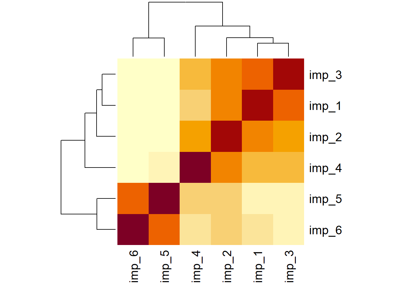
If you’re like Elizabeth and you have a hard time making sense of a matrix full of numbers, then the function heatmap() might be your friend. It represents the correlation matrix as colours. Cells representing strong positive correlations appear darker, and cells representing strong negative correlations appear lighter.
cor(gdat[,2:7]) |>heatmap()
There’s a dark diagonal line down the middle, which represents the perfect correlation between an item and itself. The cells at the intersections of Q5 and Q6 are fairly dark, and the cells at the intersections of Q1–Q4 are also fairly dark (the positive correlations). Where Q5 and Q6 meet Q1–Q4, the cells are fairly light (the negative correlations). In addition to the bracketing structure at the plot margins (in technical terms a “dendrogram”), this visual approach to a correlation matrix shows that Q5 and Q6 tend to pattern together in one way, and that the other four Qs tend to pattern together in another way.
This makes sense given the way the questions are worded - if people are impulsive, they will be more likely to disagree to Q5 and Q6, but agree with the others:
qitems
[1] "I often act on the spur of the moment without thinking."
[2] "I find it hard to resist temptations."
[3] "I make decisions quickly, even when they have serious consequences."
[4] "I find it hard to stay focused on tasks that take a long time to finish."
[5] "I prefer safe activities rather than risky things just for fun."
[6] "I am usually patient and can wait for what I want."
Question 3
Reverse score questions 5 and 6, and then examine how the correlation matrix has changed.
Be careful!! if you have some code that reverse scores a question, and you run it twice, you will essentially reverse-reverse score the question, and it goes back to the original ordering!
Solution 3. There’s only 2, so let’s do this individually for each question:
Is greater impulsivity associated with bigger losses when comparing online gamblers to casino gamblers?
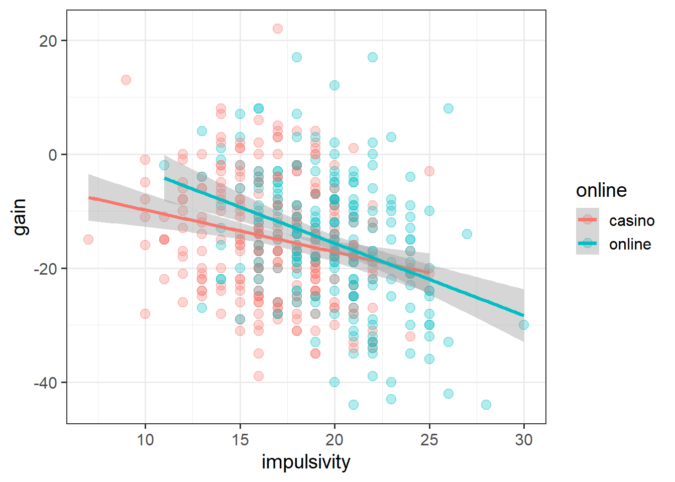
Using the scale scores that you just computed, create a plot to show how impulsivity is associated with gains/losses of gamblers in the two places (casino vs online).
Based on the plot you make, what do you predict the coefficients from the model below will look like (where impulsivity is the scale score). Will the sign of each coefficient be positive or negative?
lm(gain ~ impulsivity * online)
Once you’ve made a good effort to predict the answers to these questions, fit the model and see if your predictions are borne out. (If your predictions are different from the outcomes, reflect on why the outcomes are the way they are.)
Solution 5. Something like this should do the trick:
mod1 <-lm(gain ~ online * impulsivity, data = gdat)
It’s going to estimate 4 things:
estimate
prediction
explanation
intercept
around zero/slightly negative
the 'online' variable is coded with casino as the reference level, so the intercept is going to be the height of the casino line where impulsivity is 0. so it looks like it will be around 0, or a bit below.
onlineonline
positive
this coefficient will tell us the difference between casino and online when impulsivity is zero. the blue line in the plot is going to be higher than the red line when impulsivity is zero, so this coefficient will be positive
impulsivity
negative
this is going to be how gains/losses change when impulsivity increases, specifically for the casino group. so in my plot it is the slope of the red line. it's going to be decreasing
onlineonline:impulsivity
negative
this is going to be how the association between impulsivity and gains/losses changes when we move from casino to online. We know this association is negative in the casino group, and the online group looks like it is even more steeply downwards, so this is going to be a negative coefficient
Take a look again at the wordings of the questions on impulsivity. Do you think they equally represent the construct of ‘impulsivity’?
If you’re stuck, think about whether each question might be measuring something else, in addition to (or instead of?) impulsivity.
variable
description
imp_1
I often act on the spur of the moment without thinking.
imp_2
I find it hard to resist temptations.
imp_3
I make decisions quickly, even when they have serious consequences.
imp_4
I find it hard to stay focused on tasks that take a long time to finish.
imp_5
I prefer safe activities rather than risky things just for fun.
imp_6
I am usually patient and can wait for what I want.
Hints
This is a very subjective question. “Impulsivity” will mean subtly different things to each one of us. The idea is that we want to get at whatever idea it is that is shared across us when we use this word. To me, one of these questions feels a little less closely linked to being an ‘impulsive’ behaviour than the others.
Solution 6. I’m going to rank them in order of how much I think each question captures “impulsivity” to me.
I hope that some of you disagree with me about this ranking - that’s what makes measurement frustrating fun!
variable
description
my_thoughts
imp_1
I often act on the spur of the moment without thinking.
clearly impulsivity
imp_3
I make decisions quickly, even when they have serious consequences.
could be impulsivity, could be that you're really good at making decisions
imp_6
I am usually patient and can wait for what I want.
similar to imp_2, impatience and impulsivity kind of go hand in hand, but this is not quite so clearly the definition of impulsivity as the first two
imp_2
I find it hard to resist temptations.
'temptations' here makes me immediately think of edible temptations! which is one manifestation of impulsivity i guess!
imp_5
I prefer safe activities rather than risky things just for fun.
is risk taking the same as impulsivity? you can take calculated risks? people do 'risky' sports like climbing for fun, but not out of impulsivity?
imp_4
I find it hard to stay focused on tasks that take a long time to finish.
this doesn't really feel like it is as clearly impulsivity. lots of things can distract us from tasks. boredom?
Question 7
Okay, so if we’re not very happy that our 6 questions are equally representative of “impulsivity” (or maybe groups of questions capture distinct aspects of the construct?), we might not want to work with the plain old sum of impulsivity scores that we used above.
What are we going to do?
Let’s start by doing a Principal Component Analysis (PCA) on the 6 original items, and extracting 6 components.
Principal Components Analysis
Call: principal(r = gdat[, 2:7], nfactors = 6, rotate = "none")
Standardized loadings (pattern matrix) based upon correlation matrix
       PC1   PC2   PC3   PC4   PC5   PC6 h2       u2 com
imp_1 0.78 -0.38 -0.09  0.10 -0.32  0.35  1 -4.4e-16 2.4
imp_2 0.66  0.16 -0.66  0.19 -0.08 -0.26  1 -1.1e-15 2.6
imp_3 0.76 -0.31 -0.07 -0.16  0.54  0.06  1 -8.9e-16 2.3
imp_4 0.41  0.87  0.04  0.07  0.10  0.24  1  5.6e-16 1.7
imp_5 0.67 -0.05  0.56  0.45  0.01 -0.19  1 -1.1e-15 2.9
imp_6 0.73  0.14  0.23 -0.56 -0.22 -0.17  1 -4.4e-16 2.5

                       PC1  PC2  PC3  PC4  PC5  PC6
SS loadings           2.78 1.04 0.81 0.59 0.46 0.32
Proportion Var        0.46 0.17 0.14 0.10 0.08 0.05
Cumulative Var        0.46 0.64 0.77 0.87 0.95 1.00
Proportion Explained  0.46 0.17 0.14 0.10 0.08 0.05
Cumulative Proportion 0.46 0.64 0.77 0.87 0.95 1.00

Mean item complexity =  2.4
Test of the hypothesis that 6 components are sufficient.

The root mean square of the residuals (RMSR) is  0
 with the empirical chi square  0  with prob <  NA

Fit based upon off diagonal values = 1
Question 8
Take a look at the ‘variance accounted for’ by each component (you could use a scree plot to show this too!), and think back to our research question, which has absolutely nothing to do with whether “impulsivity” is one thing, or two things, or 6 things…
Solution 8. Our research question, remember is asking “is greater impulsivity associated with bigger losses when comparing online gamblers to casino gamblers?”
We’re getting bogged down in the weeds of what do we even mean by ‘impulsivity’?? I would make a case that our research question kind of pre-supposes that “impulsivity” is just one thing. If we reduce these 6 questions down to two or more things, then our research question becomes a little bit more complex to answer, with lots of nuance about what sort of impulsivity we’re talking about. So from a purely pragmatic standpoint, I am really hoping we can just keep one thing, and call that thing “impulsivity”!
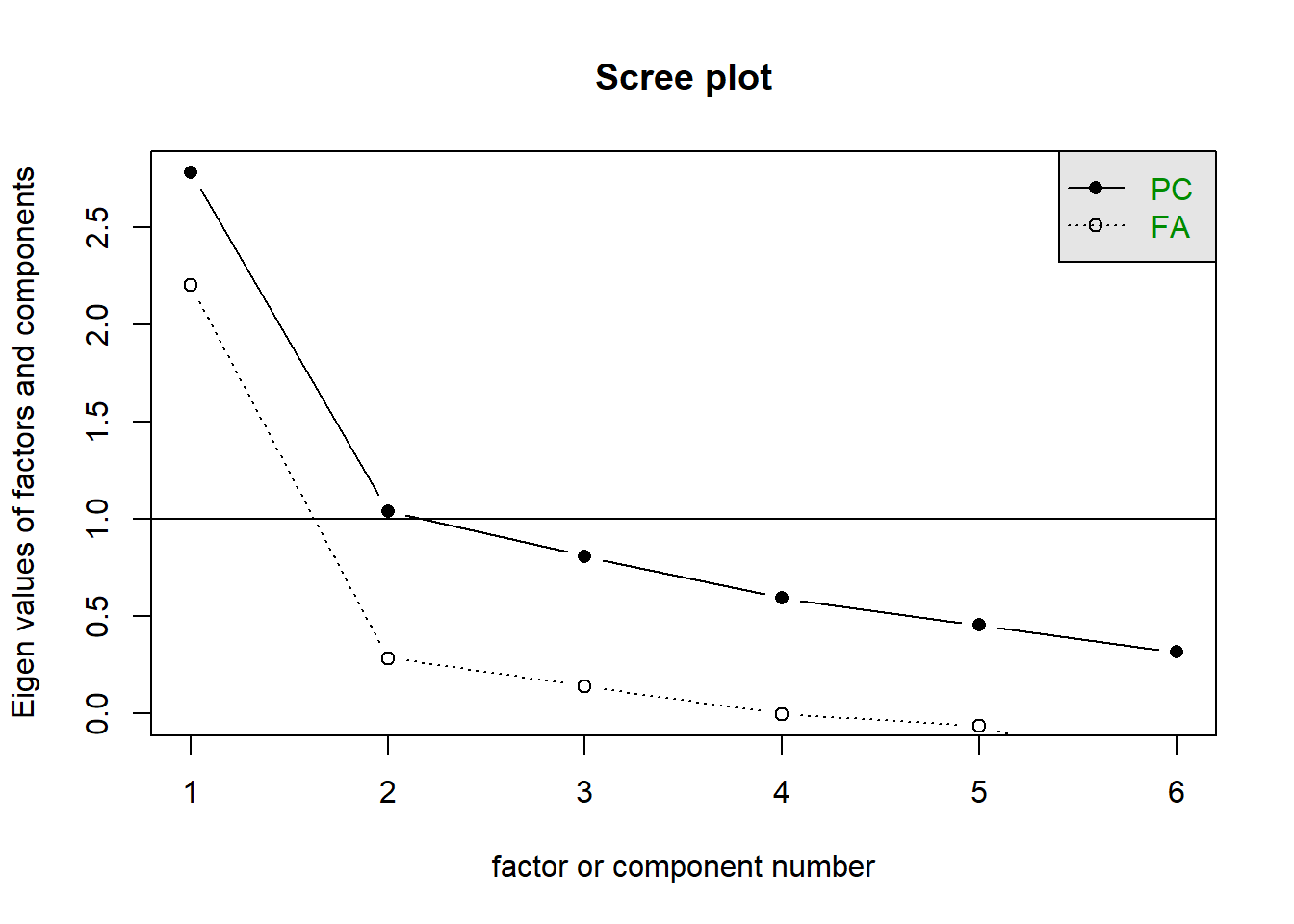
As it stands, the scree plot is in our favour. It shows a kink (or ‘elbow’, if you’d prefer) at 2 components, suggesting that we would be fine to keep just one.
scree(gdat[,2:7])
The numbers going into the scree plot are shown in the ‘variance accounted for’ bit of the PCA. These tell us that if we keep just one component, then we are capturing 47% of the variability in the questionnaire. If we kept two, then we would capture 64%, 3 would capture 77%, and so on, until we just keep 6 and we’re capturing 100%.
There’s no “right” answer here as to how much we should keep. 47% makes it feel like we’re losing more than we’re capturing (which we are), but that might just be what we have to do!
Question 9
Extract the scores for the first principal component, and attach them to your dataset as a new set of scores for “impulsivity”.
Attend also to the loadings for that first component - is it related more to the questions you felt were more clearly asked about ‘impulsivity’?
🗂️ See the How to: Get PCA Scores flash card for all things conducting PCA and extracting scores.
Solution 9. Here are the scores added to our data:
gdat$pc1 <- imppca$scores[,1]
And here are the loadings for that first component. It’s less related to imp_4 and imp_2, and more related to imp_1 and imp_3 (this kind of fits in with my view that these two questions are more obviously asking about “impulsivity” to me).
The nice result of this is that, if we use these scores and loadings in subsequent analyses, the questions that are better at targeting the construct we care about are going to be weighted more heavily than the questions that are worse at targeting that construct. The PCA scores are therefore a more accurate way of representing impulsivity than the un-weighted summed score we computed above.
Question 10
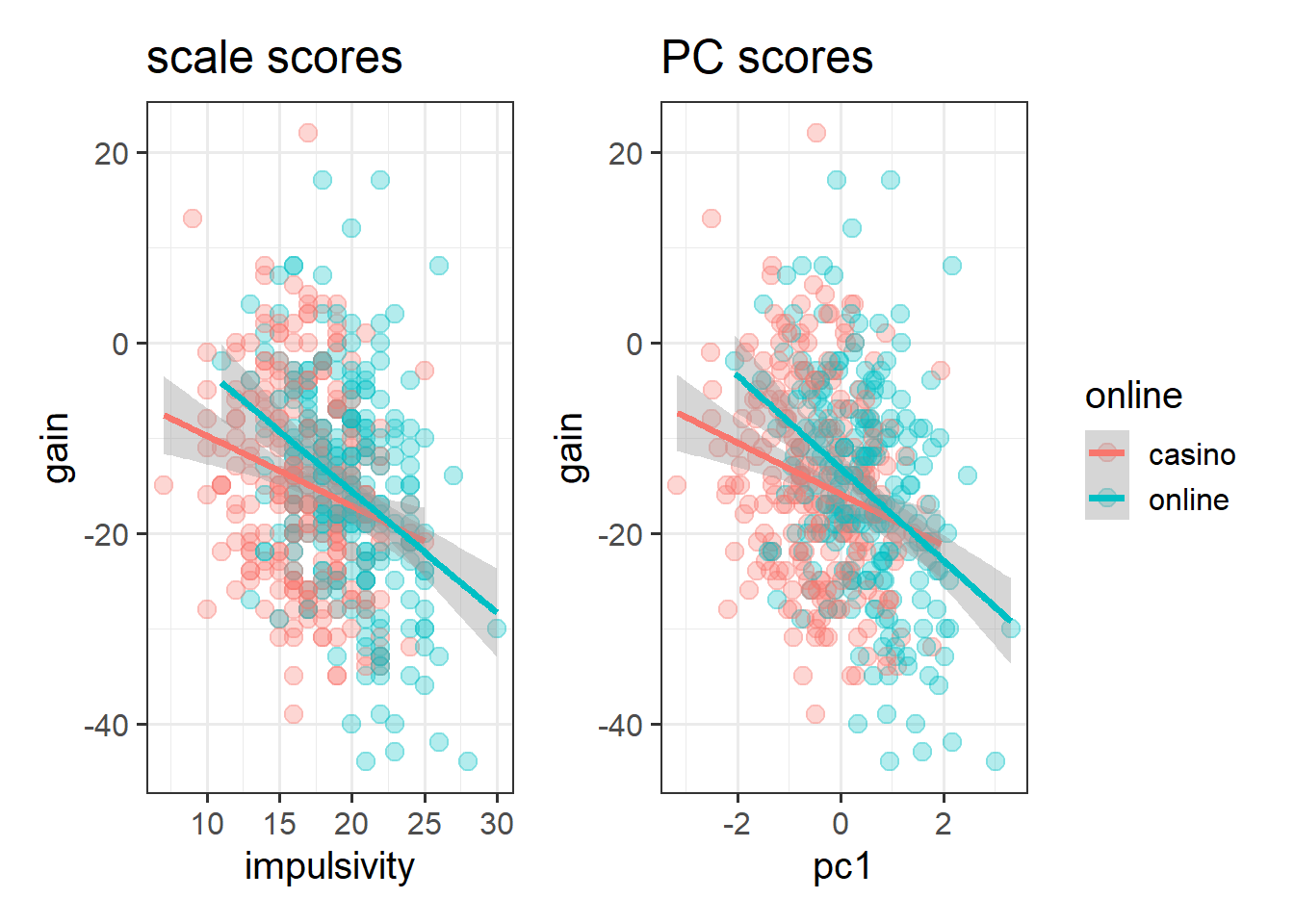
Using your PCA scores, not the old summed scale scores, create a plot that shows the association between impulsivity and financial loss or gain in the two different locations (casino and online). What changes, compared to the old plot?
Next, fit a new linear model that uses the PCA scores, not the old summed scale scores, to address the question of how impulsivity might affect gains in different locations. What changes, compared to the previous model that used the summed scale scores?
There are more different pc1 values than there are different scale score values. The scale score values can only be integers (that is, whole numbers), while the pc1 values can be decimal numbers too. This makes sense, because if the principal component scores are differentially weighting each variable, then we’re going to end up with far more possible scores.
mod2 <-lm(gain ~ online * pc1, data = gdat)sjPlot::tab_model(mod1, mod2)
gain
gain
Predictors
Estimates
CI
p
Estimates
CI
p
(Intercept)
-2.41
-9.27 – 4.44
0.489
-15.91
-17.32 – -14.51
<0.001
online [online]
12.19
1.26 – 23.12
0.029
2.72
0.68 – 4.75
0.009
impulsivity
-0.74
-1.14 – -0.34
<0.001
online [online] ×
impulsivity
-0.53
-1.12 – 0.05
0.074
pc1
-2.70
-4.09 – -1.30
<0.001
online [online] × pc1
-2.16
-4.19 – -0.12
0.038
Observations
482
482
R2 / R2 adjusted
0.091 / 0.085
0.105 / 0.099
Note that the better measurement of “impulsivity” by the PCA (weighting our scores more towards imp_1 and imp_3) results in a significant interaction here.
It’s also worth noting that the online [online] coefficient in the new model is also significant, but that is because the PCA scores are standardised, whereas the scale scores are not. So “0” means something very different on those two measures.