Troubleshooting, checking assumptions and diagnostics

In this lab, you’ll start with the maximal model you developed last week for the clothing dataset. The questions will guide you through troubleshooting the model, and once you have a version that fits, you’ll practice checking assumptions and diagnostics.

Get set up

1. Create a new .Rmd file for this week’s exercises.
2. Save it somewhere you can find it again.
3. Give it a clear name (for example, dapr3_lab04.Rmd).
4. In the first code chunk, load the packages you’ll need this week:
   • tidyverse
   • lme4
   • lmerTest
   • HLMdiag

---

Read in the dataset located at https://uoepsy.github.io/data/dapr3_mannequin.csv and name it clothing.

RQ: Are people more likely to purchase clothing when they see it displayed on a model, and is this association dependent on item price?

variable	description
purch_rating	Purchase rating (sliding scale 0 to 100, with higher ratings indicating greater perceived likelihood of purchase)
price	Price presented for item (range £5 to £100)
ppt	Participant identifier
condition	Whether items are seen on a model or on a white background

More detail about this dataset

Thirty participants were presented with a set of pictures of items of clothing, and rated each item how likely they were to buy it. Each participant saw 20 items, ranging in price from £5 to £100. 15 participants saw these items worn by a model, while the other 15 saw the items hanging against a white background.

From the Week 3 lab, here’s the maximal model for this data and RQ:

purch_rating ~ price * condition + (1 + price | ppt)

Fit the model

Question 1

The following code aims to fit the maximal model. Copy and run this code.

clothing_m1 <- lmer(
  purch_rating ~ price * condition + (1 + price | ppt), 
  data = clothing
)

What warning messages do you get? What problems do these warning messages indicate?

🗂️ See Troubleshoot common issues flash card.

Upon running that code, I get the following two warning messages:

Warning in checkConv(attr(opt, "derivs"), opt$par, ctrl = control$checkConv,  :
  Model failed to converge with max|grad| = 8.80186 (tol = 0.002, component 1)
  See ?lme4::convergence and ?lme4::troubleshooting.
Warning in checkConv(attr(opt, "derivs"), opt$par, ctrl = control$checkConv,  :
  Model is nearly unidentifiable: very large eigenvalue
 - Rescale variables?

The first warning message (the first three lines) tells me that the model failed to converge. This tells me that I might need to change the optimiser.

The second warning message (the second three lines) tells me that the model is struggling with the scale of the variables. The only predictor that has large values is price, so this tells me that I might need to rescale it (that is, transform it into z-scores).

Question 2

Change the model’s optimiser to bobyqa and re-fit the model (call it clothing_m2).

What warning messages do you see now?

🗂️ See Change optimiser flash card.

clothing_m2 <- lmer(
  purch_rating ~ price * condition + (1 + price | ppt), 
  data = clothing,
  control = lmerControl(optimizer = "bobyqa")
)

Warning in checkConv(attr(opt, "derivs"), opt$par, ctrl = control$checkConv,  :
  Model is nearly unidentifiable: very large eigenvalue
 - Rescale variables?

The bobyqa optimiser has solved the convergence problem (that first message about “Model failed to converge” has gone away). But we’re still getting the suggestion to rescale variables.

Question 3

We’ll have to rescale the predictor. Changing that might solve the convergence issue too.

• Convert price into a z-score and call the new variable price_z.
• Check that the mean of price_z is 0 and that the standard deviation is 1.
• In the code to fit clothing_m1, replace price with price_z and re-fit the model (call it clothing_m3).
• Are there any warning messages or other indications of singularity?

🗂️ See DAPR2’s Data transformations > Standardisation flash card.

See also Troubleshoot common issues flash card.

Convert price into a z-score and call the new variable price_z:

clothing <- clothing |>
  mutate(
    price_z = (price - mean(price)) / sd(price)
  )

Check that the mean of price_z is 0 and that the standard deviation is 1:

mean(clothing$price_z)

[1] 0

sd(clothing$price_z)

[1] 1

In the code to fit clothing_m1, replace price with price_z and re-fit the model (call it clothing_m3).

clothing_m3 <- lmer(
  purch_rating ~ price_z * condition + (1 + price_z | ppt),   
  # remember to also update the random slope from "price" to "price_z"!
  data = clothing
)

Are there any warning messages or other indications of singularity?

• No warning messages.
• To check other indications of singularity, we’ll need to look at the variance components of the model. We want to make sure that the SDs aren’t 0 and the correlations aren’t –1 or 1:

VarCorr(clothing_m3)

 Groups   Name        Std.Dev. Corr 
 ppt      (Intercept)  5.10         
          price_z      2.44    -0.30
 Residual             12.17         

Looks fine! The model is good to go.

Check assumptions

Question 4

Let’s move on to checking clothing_m3’s assumptions.

Are you satisfied with the assumption that the association between predictor and outcome is sufficiently linear?

🗂️ See Check assumptions flash card.

We assess linearity in LMMs using a residuals-vs-fitted plot. We want the wobbly blue line to match the horizontal black line.

plot(clothing_m3, 
     type=c(
       "p",      # includes points representing Pearson residuals
       "smooth"  # includes smoothed line representing mean of residuals
       )
    )

Good match. I’d be satisfied that the association is sufficiently linear.

Question 5

Are you satisfied with the assumption that the errors are independent?

🗂️ See Check assumptions flash card.

Our model has the maximal random effect structure licensed by the data, so yes, we can be satisfied that the errors are independent.

(Even if we had to simplify the model in order to get it to converge, we can still assume that errors are sufficiently independent.)

Question 6

Are you satisfied with the assumption that the errors are normally distributed?

🗂️ See Check assumptions flash card.

We assess normality of errors using a Q-Q plot. We want the points to match the diagonal black line.

qqnorm(resid(clothing_m3)); qqline(resid(clothing_m3))

It’s a pretty good match here. I’m satisfied that the errors are sufficiently normally distributed.

Question 7

Are you satisfied with the assumption that the errors have equal variance?

🗂️ See Check assumptions flash card.

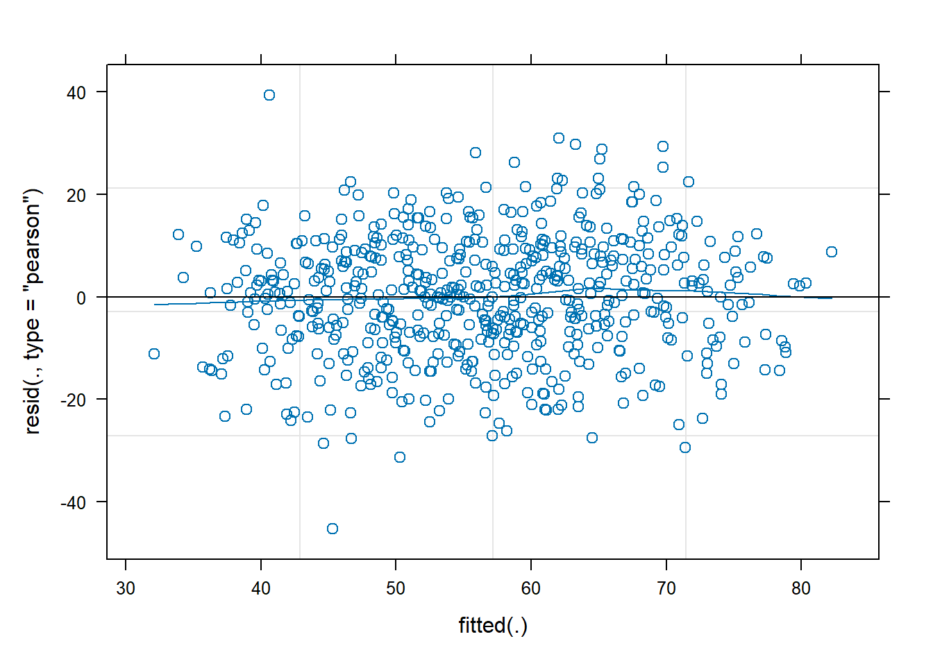
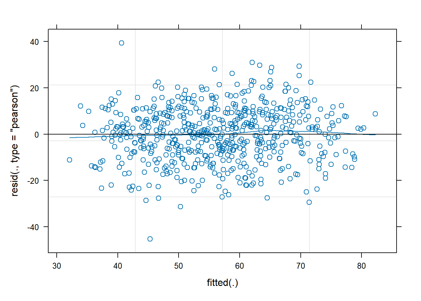
Along with linearity, we also assess equal variance of errors using a residuals-vs-fitted plot. We want the cloud of data points to have a similar vertical distance from bottom to top across the whole range of the x axis (i.e., across the range of fitted values).

plot(clothing_m3, 
     type=c(
       "p",      # includes points representing Pearson residuals
       "smooth"  # includes smoothed line representing mean of residuals
       )
    )

This cloud of data points has a pretty even vertical spread. I’d be satisfied that the residuals have equal enough variance.

Question 8

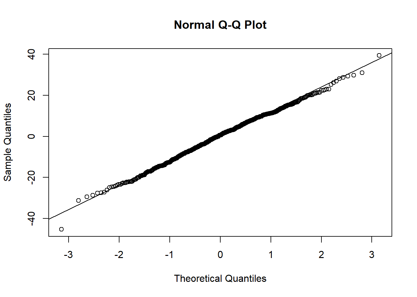
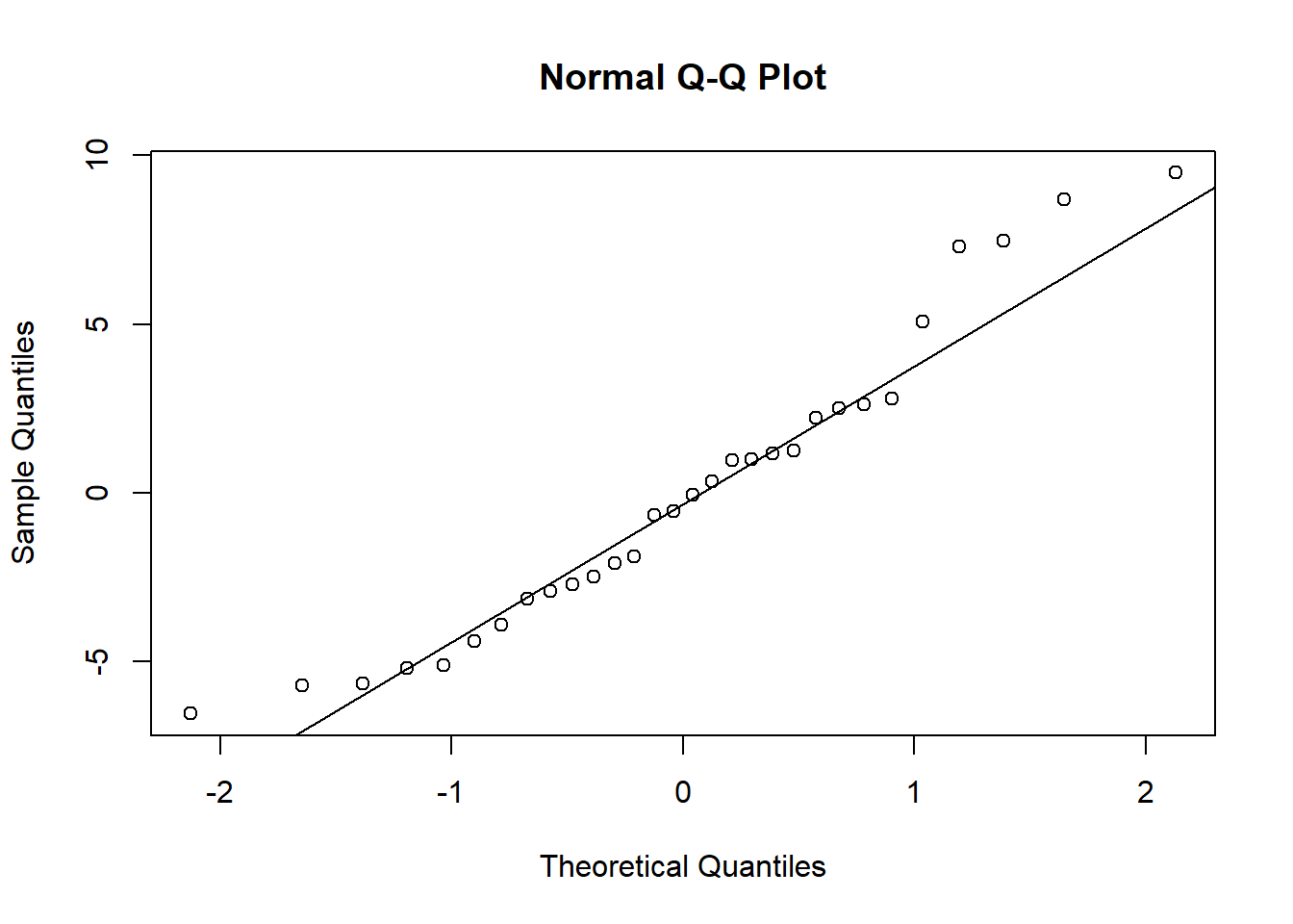
Are you satisfied with the assumption that each set of participant-level adjustments is normally distributed?

🗂️ See Check assumptions flash card.

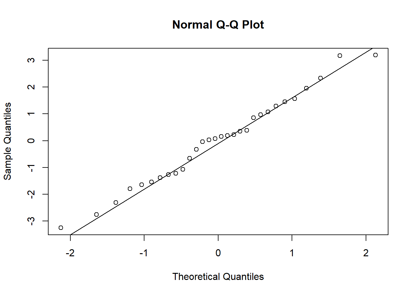
We have to check the normality of each set of by-participant adjustments individually. That is, we’ll check the participant-level intercept adjustments and separately we’ll check the participant-level slope adjustments. For both, we can use a Q-Q plot again.

The intercept adjustments:

qqnorm(ranef(clothing_m3)$ppt[,1]); qqline(ranef(clothing_m3)$ppt[,1])

The points are an OK match to the diagonal, though the extremes (the lower and upper ends) diverge a bit.

This divergence is worth commenting on in a write-up, because when we use the SD to summarise these adjustments, the SD measure works under the assumption that the data we’re summarising is approximately normal. So when it diverges a bit from normality, like here, then the SD might not be doing a perfect job capturing the variability in the data. But it’s the best we’ve got! So all we can do is report it and mention that we should be a little bit cautious in its interpretation because the by-participant intercept adjustments appear not to be perfectly normally distributed.

The slope adjustments:

qqnorm(ranef(clothing_m3)$ppt[,2]); qqline(ranef(clothing_m3)$ppt[,2])

These points are a pretty good match to the diagonal overall! I’m satisfied that the by-participant slope adjustments are sufficiently normal.

Check influence diagnostics

Question 9

Let’s move on to the influence diagnostics.

Compute and plot the approximate Cook’s Distance for each observation and for each participant.

🗂️ See Detect influential points and groups flash card.

Compute the observation-level and participant-level influence diagnostics:

inf_obs <- hlm_influence(model = clothing_m3, level = 1, approx = TRUE)
inf_ppt <- hlm_influence(model = clothing_m3, level = 'ppt', approx = TRUE)

Plot the Cook’s Distance of each observation:

dotplot_diag(inf_obs$cooksd, cutoff = "internal")

Plot the Cook’s Distance of each participant:

dotplot_diag(inf_ppt$cooksd, index = inf_ppt$ppt, cutoff = "internal")

Question 10

One of those diagnostic checks from Q9 reveals a particularly high-influence unit.

Run a sensitivity analysis to check whether this unit impacts the pattern of results and changes the conclusions we would draw from this model.

🗂️ See Detect influential points and groups flash card.

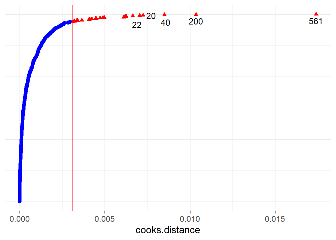
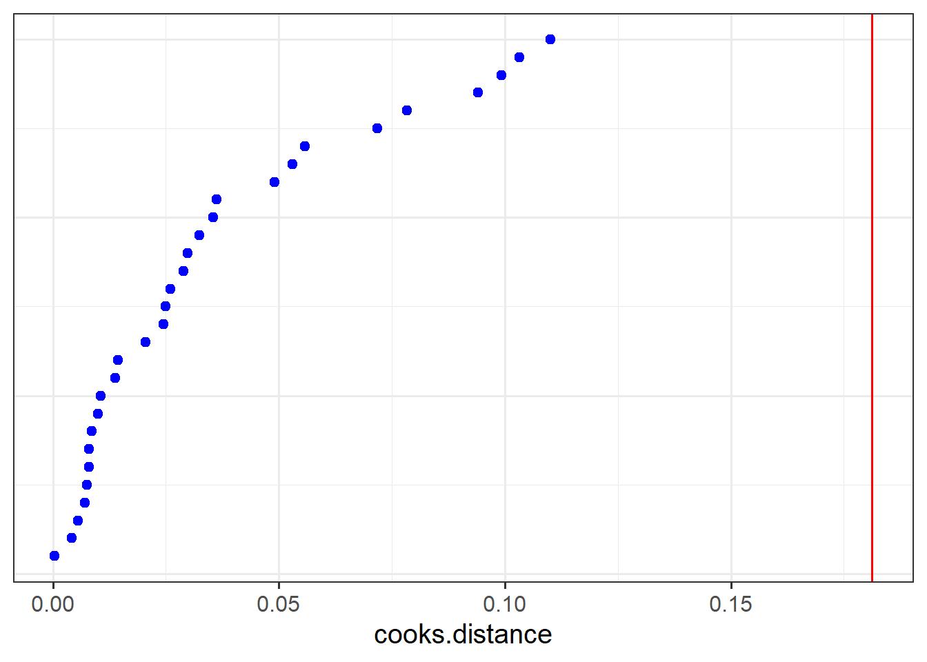
The particularly high-influence unit is in the observation-level plot, observation number 561. (No participants exert an influence above the internal Cook’s Distance threshold.)

What is observation 561?

clothing[561,]

# A tibble: 1 × 5
  purch_rating price ppt    condition price_z
         <dbl> <dbl> <chr>  <chr>       <dbl>
1           80     5 ppt_29 model       -1.65

OK, looks like participant 29 saw an inexpensive piece of clothing on a model and said that they’d be very likely to purchase it. Does this one observation drive the estimates that the model has made?

To find out, we’ll fit a new model to a version of clothing with this observation removed:

clothing_m3_no561 <- lmer(
  purch_rating ~ price_z * condition + (1 + price_z | ppt),
  data = clothing[-561,]
)

And we’ll compare the model summaries. We’re looking specifically for big differences in the fixed effect coefficients and in their statistical significance.

summary(clothing_m3)

Linear mixed model fit by REML. t-tests use Satterthwaite's method [
lmerModLmerTest]
Formula: purch_rating ~ price_z * condition + (1 + price_z | ppt)
   Data: clothing

REML criterion at convergence: 4750

Scaled residuals: 
   Min     1Q Median     3Q    Max 
-3.724 -0.639  0.049  0.684  3.235 

Random effects:
 Groups   Name        Variance Std.Dev. Corr 
 ppt      (Intercept)  25.97    5.10         
          price_z       5.94    2.44    -0.30
 Residual             148.04   12.17         
Number of obs: 600, groups:  ppt, 30

Fixed effects:
                       Estimate Std. Error     df t value Pr(>|t|)    
(Intercept)              54.283      1.492 28.000   36.39   <2e-16 ***
price_z                   7.147      0.943 28.000    7.57    3e-08 ***
conditionmodel            4.237      2.109 28.000    2.01    0.054 .  
price_z:conditionmodel    3.347      1.334 28.000    2.51    0.018 *  
---
Signif. codes:  0 '***' 0.001 '**' 0.01 '*' 0.05 '.' 0.1 ' ' 1

Correlation of Fixed Effects:
            (Intr) pric_z cndtnm
price_z     -0.179              
conditinmdl -0.707  0.126       
prc_z:cndtn  0.126 -0.707 -0.179

summary(clothing_m3_no561)

Linear mixed model fit by REML. t-tests use Satterthwaite's method [
lmerModLmerTest]
Formula: purch_rating ~ price_z * condition + (1 + price_z | ppt)
   Data: clothing[-561, ]

REML criterion at convergence: 4732

Scaled residuals: 
   Min     1Q Median     3Q    Max 
-3.767 -0.639  0.057  0.688  2.571 

Random effects:
 Groups   Name        Variance Std.Dev. Corr 
 ppt      (Intercept)  26.43    5.14         
          price_z       6.58    2.57    -0.32
 Residual             144.77   12.03         
Number of obs: 599, groups:  ppt, 30

Fixed effects:
                       Estimate Std. Error    df t value Pr(>|t|)    
(Intercept)               54.28       1.50 27.99   36.23  < 2e-16 ***
price_z                    7.15       0.96 27.86    7.44  4.3e-08 ***
conditionmodel             4.09       2.12 28.02    1.93    0.064 .  
price_z:conditionmodel     3.59       1.36 28.00    2.64    0.013 *  
---
Signif. codes:  0 '***' 0.001 '**' 0.01 '*' 0.05 '.' 0.1 ' ' 1

Correlation of Fixed Effects:
            (Intr) pric_z cndtnm
price_z     -0.193              
conditinmdl -0.707  0.136       
prc_z:cndtn  0.136 -0.706 -0.194

The coefficients are pretty similar. And the pattern of statistical significance does not change at all.

Therefore we can conclude that, although observation 561 has the highest Cook’s Distance out of all the observations, it doesn’t hugely influence the model’s estimates nor change the conclusions we would draw from the analysis.