LMMs: Practice write-up

In this lab, you’ll be guided through how to report the LMM analysis we conducted together in lectures this week.

Your goal is for a reader to be able to replicate your analyses in any software they choose, based only on what you’ve written.

Make sure that your write-up contains no visible R code. For a reminder of how to hide code, format tables, etc., check out the DAPR1 formatting resources.

Get set up

1. Create a new .Rmd file for this week’s exercises.
2. Save it somewhere you can find it again.
3. Give it a clear name (for example, dapr3_lab05.Rmd).

The RQ and the data

Study background:

• We’re looking at emotional dysregulation in children: when children have trouble managing their feelings and emotions.
• Specifically, we want to find out how emotional dysregulation is affected by children having a strong, regular routine at home.
• We predict that children with stronger home routines are better at regulating their emotions.
• It’s also plausible that a family’s socio-economic status (SES) is associated with how well children regulate their emotions. We will control for SES using a proxy variable of whether children attend a state school or a private school.

RQ: Controlling for the type of school that children attend, are children with stronger routines better at regulating their emotions?

The data can be downloaded from https://uoepsy.github.io/data/crqeds.csv.

variable	description
schoolid	School identifier
EDS	Emotion Dysregulation Score (range 1 to 6, higher values indicate more dysregulation)
CRQ	Childhood Routine Questionnaire Score (range 0 to 7, higher values indicate more routine)
schooltype	School type (private / state)

Provided analysis code

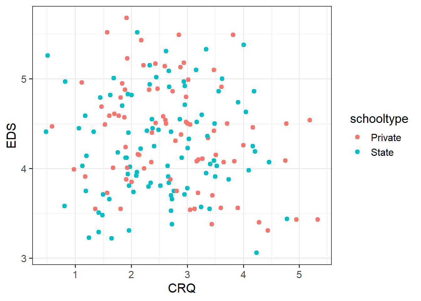
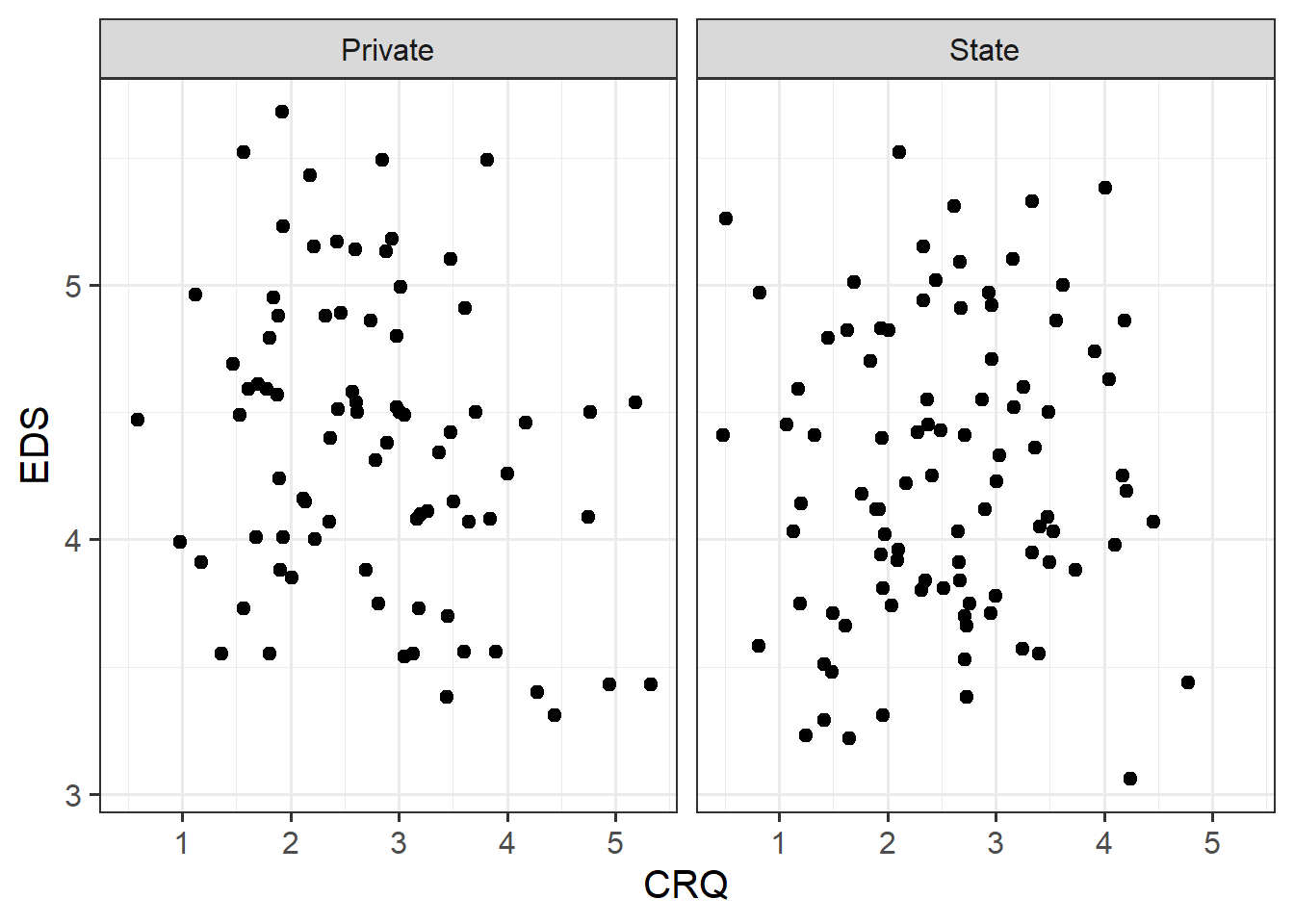
# LMMs: Practice analysis
# Example code 

# PHASE 1 ----

## 1a: Set up code and data ----

# Load required R packages
library(tidyverse)
library(lme4)
library(lmerTest)
library(stats)
library(HLMdiag)
library(effects)
library(car)

# Read in data
eds_data <- read_csv("https://uoepsy.github.io/data/crqeds.csv")

# Tidy data
glimpse(eds_data)

summary(eds_data$EDS)
summary(eds_data$CRQ)
table(eds_data$schoolid)
table(eds_data$schooltype)

is.na(eds_data) |> table()


## 1b: Set up fixed effects ----

# Identify outcome + predictors:
# RQ: Controlling for the type of school that children attend, are children with
# stronger routines better at regulating their emotions?
# - Outcome: EDS
# - Predictors: schooltype, CRQ

# Do we need an interaction?
# - No, because we're just controlling for schooltype, not looking at how 
#   different schooltypes affect the association between EDS and CRQ.

# Regular or logistic regression?
# - EDS is not a binary variable, so regular regression.

# Set up categorical predictors: schooltype.
# - Convert schooltype to factor and check ref level.
eds_data <- eds_data |>
  mutate(
    schooltype = factor(schooltype)
  )
contrasts(eds_data$schooltype)  # ref level = Private

# Set up continuous predictors: CRQ.
# - CRQ ranges from 0 to 7, so it's justifiable to leave it as-is.
# - NB: Mean-centering would also be justifiable, since no observations = 0.
eds_data$CRQ |> sort()

# Explore patterns by plotting outcome and predictor variables together.
# - one version with schooltype as colour
eds_data |>
  ggplot(aes(x = CRQ, y = EDS, colour = schooltype)) +
  geom_point()

# - another version with schooltype as facets
eds_data |>
  ggplot(aes(x = CRQ, y = EDS)) +
  geom_point() +
  facet_wrap(~ schooltype)

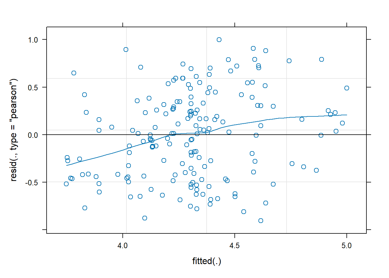
## 1c: Set up random effects ----

# Identify grouping variables that contribute random variability:
# - The only remaining variable is schoolid, so check if it is a
# - grouping variable (i.e., if each schoolid has multiple observations)
eds_data |>
  group_by(schoolid) |>
  count()
# - And we want our results to generalise over lots of schools, not just these,
#   and we could survey different schools and answer the same RQ. So, yes,
#   random variability, and therefore we'll need random intercept by schoolid.

# Describe randomly-varying grouping variables:
# - How many levels?
n_distinct(eds_data$schoolid)
# - Just computed how many children per school (see above).
# - Summary stats about how many obs per level?
eds_data |>
  group_by(schoolid) |>
  count() |>
  ungroup() |>
  summarise(
    mean_obs = mean(n),
    med_obs  = median(n),
    min_obs  = min(n),
    max_obs  = max(n)
  )

# Identify random slopes.
# - Does each level of schoolid appear with at least one value of CRQ? 
# - Yes, though the xtabs trick is a bit silly with a continuous predictor.
xtabs(~ schoolid + CRQ, data = eds_data)
# - A trick from the flash cards to count all the non-zero values per school: 
(xtabs(~ schoolid + CRQ, data = eds_data)  != 0) |> rowSums()

# Does each level of schoolid appear with at least one value of schooltype? 
# - No.
xtabs(~ schoolid + schooltype, data = eds_data)

# Maximal model formula:
# - EDS ~ schooltype + CRQ + (1 + CRQ | schoolid)


# PHASE 2 ----

# Try fitting maximal model.
eds_m1 <- lmer(
  EDS ~ schooltype + CRQ + (1 + CRQ | schoolid),
  data = eds_data
)

# No warnings, but check variance components for sneaky singularities.
VarCorr(eds_m1)
# Looks fine!


# PHASE 3 ----

## 3a: Check assumptions and diagnostics ----

# Check model assumptions:

# - Linearity of association:
plot(eds_m1, 
     type=c(
       "p",      # includes points representing Pearson residuals
       "smooth"  # includes smoothed line representing mean of residuals
     )
)

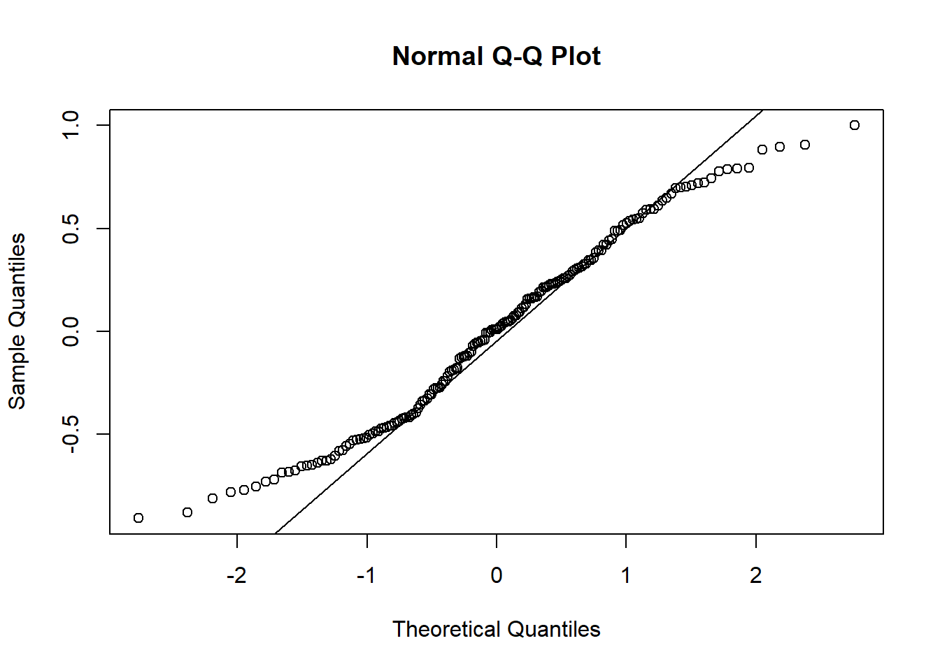
# - Linearity appears violated, but fun fact: residual-vs-fitted plots for LMMs
# - often trend upward like this, especially when there are only a few observations
# - per level of grouping variable. So not actually a cause for concern.

# - Normality of errors:
qqnorm(resid(eds_m1)); qqline(resid(eds_m1))

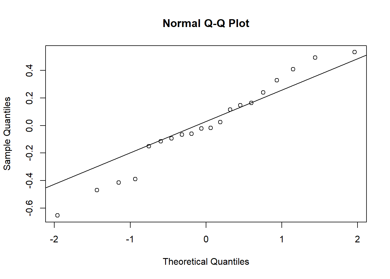
# - Some deviations at extremes.
# - This is because EDS is bounded between 1 and 6, and we see the taper that reflects this.
# - But this LMM assumes outcome is truly continuous.
# - Beyond DAPR3, there are other kinds of generalised LMs that are better for 
#   bounded data. But it's OK for now.

# - Revisit residuals-vs-fitted plot for equal variance of errors: looks fine.

# - Normality of random effects:
qqnorm(ranef(eds_m1)$schoolid[,1]); qqline(ranef(eds_m1)$schoolid[,1])

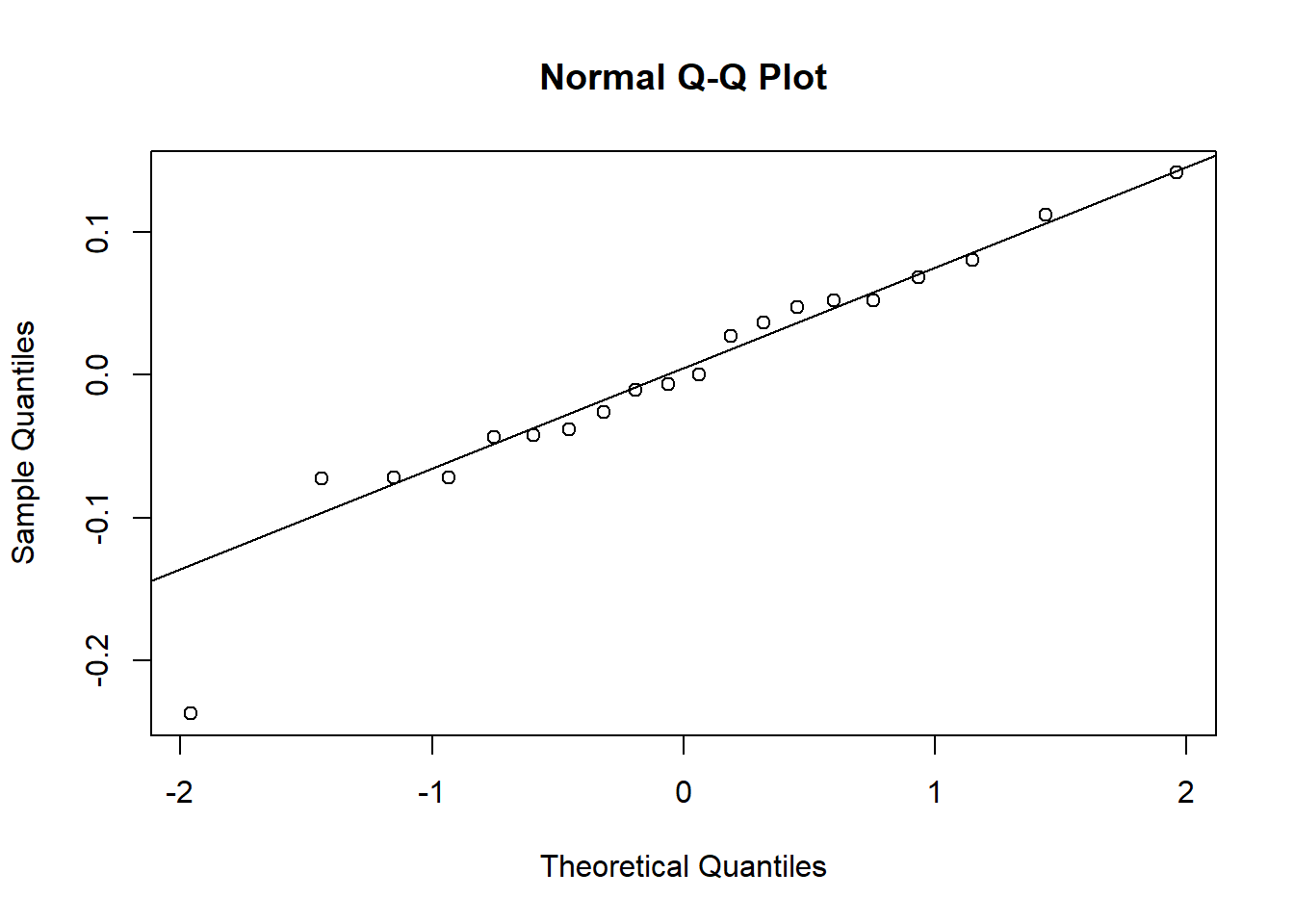
# - ^ could be better. could also be worse.
qqnorm(ranef(eds_m1)$schoolid[,2]); qqline(ranef(eds_m1)$schoolid[,2])

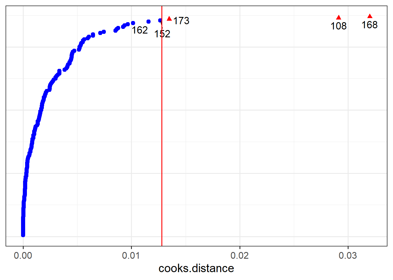
# - ^ better except for one slope adjustment being way smaller than we'd expect!
# Not perfect but OK overall.
# SD will probably be an OK representation of the spread of these adjustments.


# Run diagnostics for multicollinearity.
vif(eds_m1)  # all = 1


# Check influence of observations and schools
inf_obs      <- hlm_influence(model = eds_m1, level = 1, approx = TRUE)
inf_schoolid <- hlm_influence(model = eds_m1, level = "schoolid", approx = TRUE)

dotplot_diag(inf_obs$cooksd, cutoff = "internal")

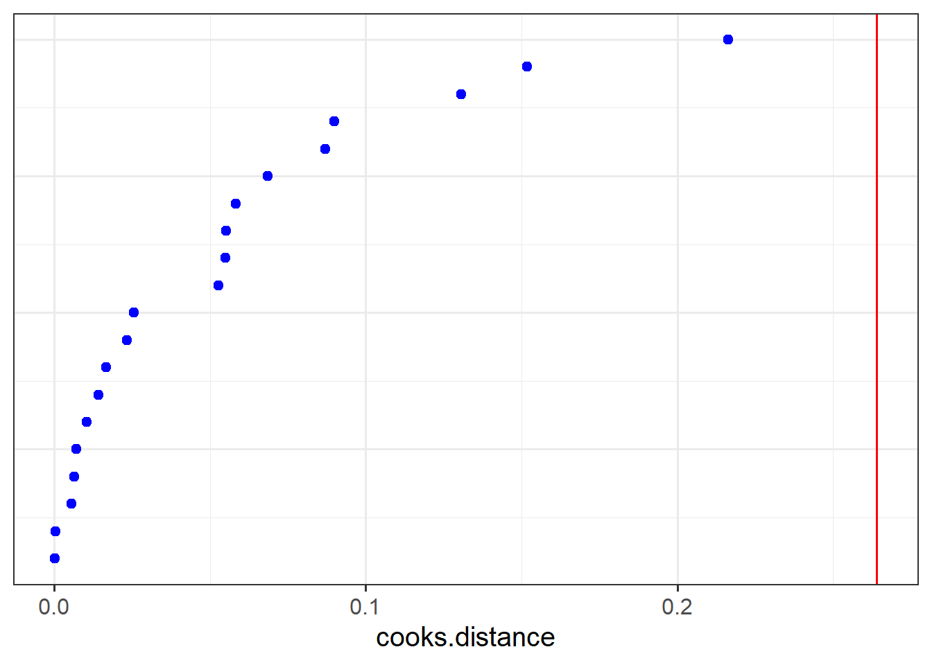
dotplot_diag(inf_schoolid$cooksd, index = inf_schoolid$schoolid, cutoff = "internal")

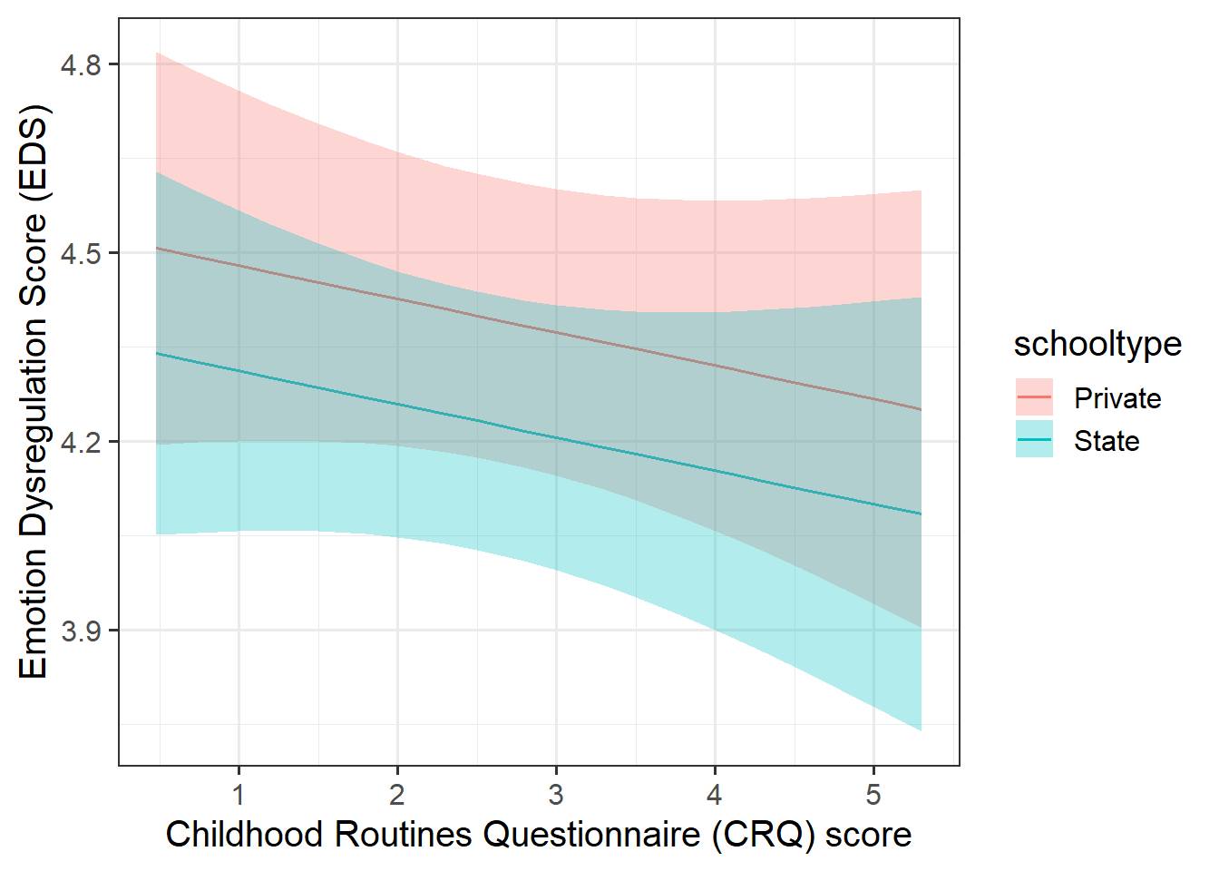
# (could consider sensitivity analysis for obs 108 and 168, 
# but skipping for reasons of time)


## 3b: Plot and interpret model estimates ----

# Plot model-fitted values:

Effect(focal.predictors = c("CRQ", 'schooltype'), mod = eds_m1) |> 
  as.data.frame()

# - CRQ is spaced weird, so we'll ask for more levels
Effect(
  focal.predictors = c("CRQ", 'schooltype'), 
  mod = eds_m1, 
  xlevels = 20  # how many levels for continuous x axis predictor
) |>
  as.data.frame() 

# - better. now plot it:
Effect(
  focal.predictors = c("CRQ", 'schooltype'), 
  mod = eds_m1, 
  xlevels = 20
) |>
  as.data.frame() |>
  ggplot(aes(x = CRQ, y = fit)) +
  geom_line(aes(colour = schooltype)) +
  geom_ribbon(aes(ymin = lower, ymax = upper, fill = schooltype), alpha = 0.3) +
  labs(
    y = 'Emotion Dysregulation Score (EDS)',
    x = 'Childhood Routines Questionnaire (CRQ) score'
  )

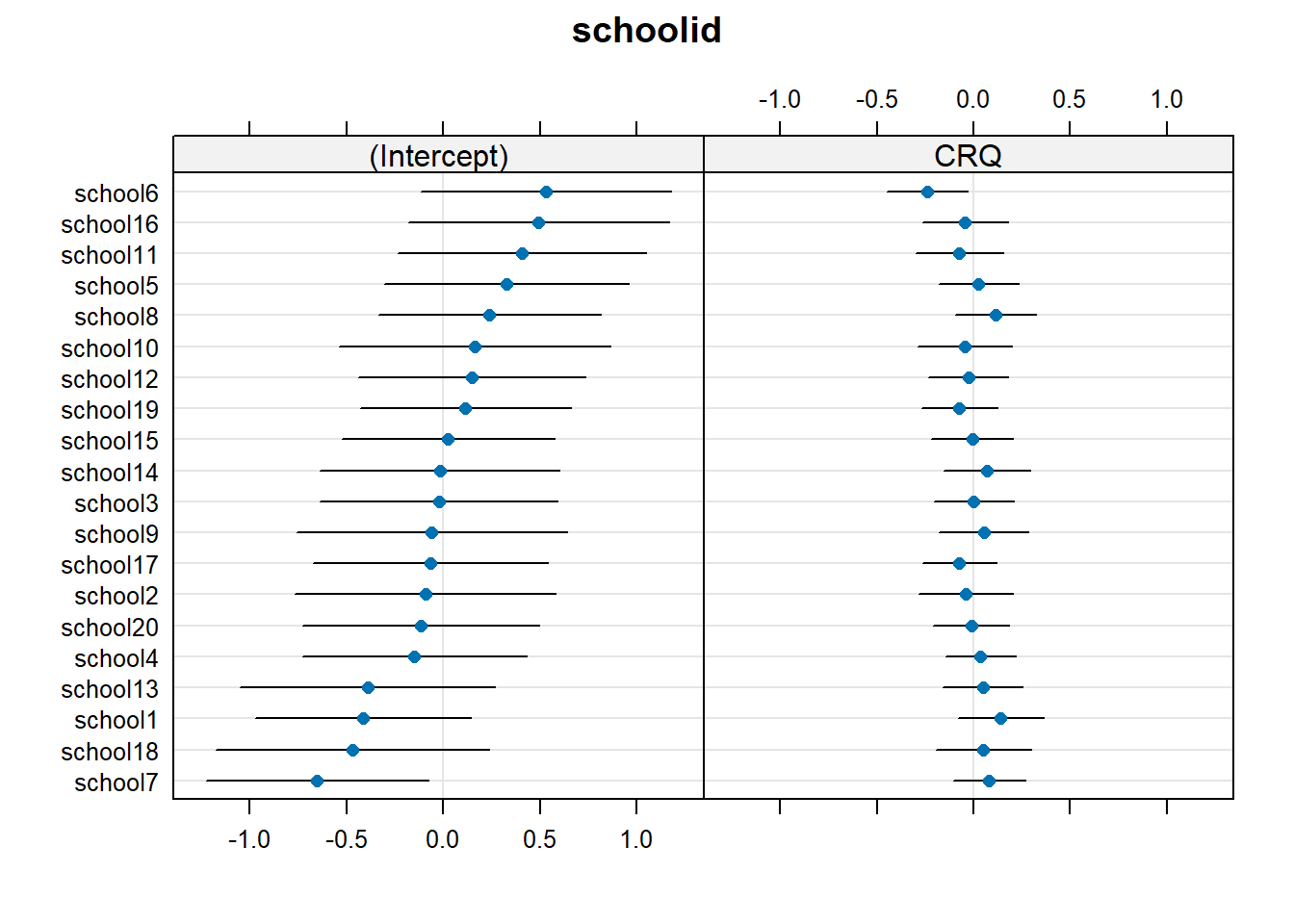
# Interpret fixed effects:
fixef(eds_m1) |> round(2)
# - Intercept: The average estimated emotional dysregulation for pupils in 
#   private schools with CRQ = 0 (that is, zero routine) is 4.53 points.
# - schooltypeState: Holding CRQ constant (ie, for any value of CRQ), moving 
#   from private schools to state schools is associated with a decrease of EDS 
#   of 0.17 points. That is, dysregulation decreases, or regulation increases.
#   This difference is not significantly different from zero.
# - CRQ: Holding school type constant (ie, for any value of school type), an 
#   increase of one CRQ point is associated with a decrease of EDS of 0.05. 
#   That is, dysregulation decreases, or regulation increases. This difference 
#   is also not significantly different from zero.
  
# Plot random effects:
dotplot.ranef.mer(ranef(eds_m1))

# Interpret SD of random effects relative to fixed effects.
VarCorr(eds_m1)
# - The by-school intercept adjustments have a SD of 0.46 points. Thus the model
#   suggests that 95% of the adjusted school-level intercepts fall between 
4.53 - 2 * 0.46 #  3.61 and 
4.53 + 2 * 0.46 #  5.45 EDS points.
# - The by-school adjustments to the slope over CRQ have a SD of 0.14 points. 
#   Thus the model suggests that 95% of the school-level slopes over 
#   CRQ – SPECIFICALLY FOR REF LEVEL, SO FOR PRIVATE SCHOOLS – fall between 
-0.05 - 2 * 0.14 #  -0.33 and 
-0.05 + 2 * 0.14 #  0.23.
#   Thus most private schools show a negative association between CRQ and EDS (meaning 
#   that as routine increases, dysregulation decreases—in line with the 
#   hypothesis), but some private schools are also estimated to show a positive 
#   association (not in line with the hypothesis).


# Interpret correlation between intercept and slope adjustments.
# - The intercept and slope adjustments have a fairly large negative correlation
#   of –0.75. This suggests that schools that tend to have students with higher 
#   emotional dysregulation scores (big intercept) tend to have a more negative 
#   adjustment to the slope of CRQ. Since this fixed slope is already negative,
#   the more negative adjustments suggest that the effect of CRQ tends to be 
#   stronger in schools with pupils having higher emotional dysregulation.

## 3c: Write up methods and results ----

---

Question 1

Set the scene (so the reader knows what you’re talking about).

• Remind the reader briefly what the study aimed to test (e.g., what the predictions were).
• Introduce the variables the study is using to test this prediction, but avoid using R variable names; describe the variables in human-readable terms instead (e.g., what scale are they on? how were they measured?)

🗂️ See Report LMM analyses and results flash card.

Solution 1. This study aimed to investigate how the strength of children’s day-to-day routines might be associated with their ability to regulate their own emotions. Researchers gathered children’s emotional dysregulation scores (EDS, ranging from 1 to 6) as well as their scores on the Childhood Routines Questionnaire (CRQ, ranging from 0 to 7). Additionally, children’s emotional dysregulation could be impacted by their family’s socio-economic status (SES), so researchers also recorded what type of school students attend (private or state) as a proxy for SES. The researchers predicted that stronger routines may be associated with lower emotional dysregulation (or in other words, better emotional regulation) in children, when controlling for school type.

Question 2

Describe and show the sample data (so that the reader knows how generalisable your analysis might be).

• If applicable, mention any data cleaning / outlier removal you did before computing the descriptives.
• Describe the data set: how many observations?
• Describe the grouping variables in your data (see Describe group-structured data).
  • Tip: If you find yourself listing loads of numbers in the text, consider using tables or plots instead (and they’re better for your word count too!).

🗂️ See Describe group-structured data flash card.

Solution 2. Researchers collected data from 174 children from 20 different schools. The median number of children sampled from each school was 9, and the number of children from each school ranged from 4 to 10.

[If we had more data about the children’s ages or genders, for example, then this would be the place to summarise that as well.]

Question 3

Visualise and summarise the results that address the RQ (so the reader knows the basic pattern of what you found).

• Include a plot of the data (and make sure to refer to it in the text).
  • Tip: If you transform any continuous predictors for analysis, use the transformed version of the predictor in the plot.
  • Tip: Academic writing styles vary, but Elizabeth likes it when figure captions give the reader a brief take-home message about what they should see in the plot.
• In a sentence or two, describe the overall pattern of results.
  • Tip: No inferential stats have been done yet, so we can’t make any claims just yet about whether the predictions were supported. But it is OK to say whether the results appear broadly in line with the prediction.

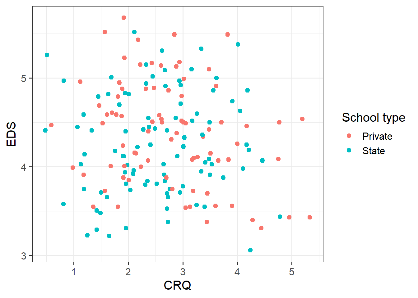
Solution 3. Relationships between children’s EDS values, their CRQ scores, and their school type are shown in Figure 1.

Figure 1. Children’s Emotional Dysregulation Score (EDS), Childhood Routines Questionnaire (CRQ) score, and their school type. No clear association between variables is apparent.

The researchers predicted that as CRQ score increases, EDS should decrease, which would appear in Figure 1 as a negative correlation between CRQ and EDS. But Figure 1 shows no obvious association between any of the variables it depicts.

Question 4

Introduce your statistical analysis (so the reader can interpret the numbers you will report).

• State that you’re running your analysis using R, and cite the developers (run citation() in the console to get the citation for your version of R).
• It’s good practice to cite the creators of lme4 and lmerTest as well. Get their information by running citation("lme4") and citation("lmerTest").
• Describe the fixed effects of your model, e.g.: “We fit a linear mixed model predicting Y as a function of X1, X2, and their interaction”.
• If categorical predictors, describe contrast coding, e.g.: “X1 has two levels, A (coded as –1) and B (coded as 1)”.
• If continuous predictors have been transformed, describe the transformation, e.g.: “X2 has been z-scored”.
• Describe the random effect structure of the maximal model.
  • One option using “random” terminology (more traditional): “The maximal model includes by-participant random intercepts, by-participant random slopes over X1, and by-stimulus random intercepts.”
  • Another option using “adjustment” terminology (less traditional but clearer): “The maximal model includes by-participant adjustments to the intercept and to the slope over X1, as well as by-stimulus intercept adjustments.”
• If you had to simplify the random effect structure, describe the order in which you removed parameters.
• Describe the random effect structure of your final model that converged without singularities (that is, describe the model that you’ll actually report below).
• State the model’s estimation method (REML or ML), how p-values were computed (if lmerTest, probably Satterthwaite’s method), what optimiser you used, …

🗂️ See Maximal model, Simplify random effects flash cards.

Solution 4. This analysis was conducted using R version 4.5.2 (R Core Team, 2025), using the packages lme4 (Bates et al., 2015) and lmerTest (Kuznetsova et al., 2017).

We fit a linear mixed model predicting EDS as a function of CRQ score and school type. School type was coded using R’s default treatment coding, with “Private” as the reference level. The maximal random effect structure for this model includes by-school adjustments to the intercept and to the slope over CRQ score. This model converged without singularities using REML estimation. The \(p\)-values we report below were computed using Satterthwaite’s method.

[Cite your version of R, not mine! And remember to include all these references in your bibliography.]

Question 5

Report the results of your analysis (so the reader knows exactly what you found).

• State which model coefficient(s) are related to which prediction(s), and what direction/sign (positive or negative) you would expect the coefficients to have if the predictions were borne out.
• State the key coefficient estimates along with their 95% CI and p-value, e.g.: “The slope associating X1 and Y was significantly different from zero (\(b\) = 0.26, 95% CI [0.23, 0.29], \(p\) < 0.001)” or “The slope associating X1 and Y was not significantly different from zero (\(b\) = 0.26, 95% CI [–0.04, 0.56], \(p\) = 0.18)”.
  • Tip: You don’t need to report every single parameter estimate. Focus on the one(s) you identified as being relevant to your prediction(s).
  • Tip: Briefly link the direction and significance of the effect back to your earlier predictions—is the prediction supported by the parameter estimate?
• Include a table of all coefficients estimated by the linear model (and make sure to refer to it in the text). The function tab_model() from the package sjPlot is useful here, but note that tab_model() causes Rmd files to fail to knit to PDF, so you might want to manually recreate the table it produces.
• Plot the model-fitted values (and refer to the plot in the text).
• Report the magnitude of the SD of the group-level adjustments and compare it to the magnitude of the fixed effects. How does the intercept vary between groups? How does the effect of interest vary between groups?
• Report the correlations between intercept and slope adjustments.
• Report any other information you consider important for your story!

🗂️ See Plot model-fitted values, Interpret LMM summary flash cards.

Solution 5. To support the researcher’s prediction, the slope associating CRQ scores with EDS should be negative. This would indicate that, as CRQ increases by one point, dysregulation would decrease (while holding school type constant).

As the regression coefficients in Table 1 show, the CRQ slope parameter is indeed negative, but it is not significantly different from zero (\(b\) = –0.05, 95% CI [–0.15, 0.05], p = 0.297). Therefore the researchers’ prediction is not supported by this analysis.

Table 1. Regression coefficients for the linear mixed model associating CRQ scores and school type with EDS in children.

	EDS
Predictors	Estimates	CI	p
(Intercept)	4.53	4.19 – 4.88	<0.001
schooltype [State]	-0.17	-0.47 – 0.14	0.280
CRQ	-0.05	-0.15 – 0.05	0.297
Random Effects
σ2	0.24
τ00 schoolid	0.21
τ11 schoolid.CRQ	0.02
ρ01 schoolid	-0.76
ICC	0.31
N schoolid	20
Observations	174
Marginal R2 / Conditional R2	0.025 / 0.326

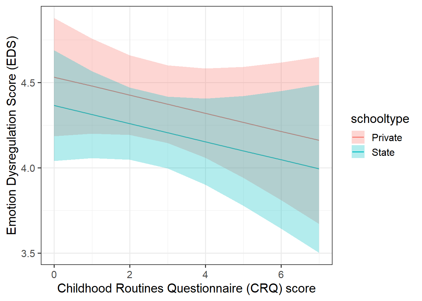
Figure 2 illustrates the model-fitted values, which on average show a negative trend, although positive trends are still compatible with the wide 95% CI ribbons.

Figure 2. Model-fitted values illustrating the estimated associations between children’s Emotional Dysregulation Score (EDS), Childhood Routines Questionnaire (CRQ) score, and their school type. Although CRQ and EDS appear negatively associated on average, no associations were found to be statistically significant.

Further, the model indicates a fair amount of variability schools in their pupils’ baseline levels of EDS and in the association between CRQ and EDS.

The model’s fixed intercept tells us that the estimated average EDS for privately-educated children with a CRQ score of zero is 4.53 points. The adjustments to this intercept that the model estimated for each school have a SD of 0.46, meaning that 95% of adjusted school-level intercepts are estimated to fall between about 3.61 and 5.45 points on the EDS scale, nearly spanning the upper half of the scale.

More crucially to the research question, the model also estimated that the school-level adjustments to the slope over CRQ score have a SD of 0.14. In other words, for private schools, about 95% of slopes over CRQ scores fall between –0.33 and 0.23: a wide range which covers both the negative association that researchers predicted and a positive association which they did not.

Finally, school-level intercept and slope adjustments have a correlation of –0.76. This correlation suggests that schools whose pupils have higher baseline EDS values (that is, larger positive intercept adjustments) tend to have larger negative slope adjustments, meaning that the already-negative slope over CRQ value would become even more strongly negative. Phrased more clearly, this suggests that in schools where pupils have higher emotional dysregulation, the effect of routine on helping students regulate their emotions may be stronger.

[Beware: sjPlot::tab_model() causes Rmd files to fail to knit to PDF. You could knit to HTML instead, or recreate the table manually, or take a screenshot of the tab_model() output and include that in your report.]