W9 Exercises: CFA

Exercises for the Enthusiastic

Dataset: radakovic_das.csv

Apathy is lack of motivation towards goal-directed behaviours. It is pervasive in a majority of psychiatric and neurological diseases, and impacts everyday life. Traditionally, apathy has been measured as a one-dimensional construct but is in fact composed of different types of demotivation.

The Dimensional Apathy Scale (DAS) is a multidimensional assessment for demotivation, in which 3 subtypes of apathy are assessed:

• Executive: lack of motivation for planning, attention or organisation
• Emotional: lack of emotional motivation (indifference, affective or emotional neutrality, flatness or blunting)
• Initiation: lack of motivation for self-generation of thoughts and/or actions

The DAS measures these subtypes of apathy and allows for quick and easy assessment, through self-assessment, observations by informants/carers or administration by researchers or healthcare professionals.

You can find data for the DAS when administered to 250 healthy adults at https://uoepsy.github.io/data/radakovic_das.csv, and information on the items is below.

DAS Dictionary

All items are measured on a 6-point Likert scale of Always (0), Almost Always (1), Often (2), Occasionally (3), Hardly Ever (4), and Never (5). Certain items (indicated in the table below with a - direction) are reverse scored to ensure that higher scores indicate greater levels of apathy.

item	direction	dimension	question
1	+	Executive	I need a bit of encouragement to get things started
2	-	Initiation	I contact my friends
3	-	Emotional	I express my emotions
4	-	Initiation	I think of new things to do during the day
5	-	Emotional	I am concerned about how my family feel
6	+	Executive	I find myself staring in to space
7	-	Emotional	Before I do something I think about how others would feel about it
8	-	Initiation	I plan my days activities in advance
9	-	Emotional	When I receive bad news I feel bad about it
10	-	Executive	I am unable to focus on a task until it is finished
11	+	Executive	I lack motivation
12	+	Emotional	I struggle to empathise with other people
13	-	Initiation	I set goals for myself
14	-	Initiation	I try new things
15	+	Emotional	I am unconcerned about how others feel about my behaviour
16	-	Initiation	I act on things I have thought about during the day
17	+	Executive	When doing a demanding task, I have difficulty working out what I have to do
18	-	Initiation	I keep myself busy
19	+	Executive	I get easily confused when doing several things at once
20	-	Emotional	I become emotional easily when watching something happy or sad on TV
21	+	Executive	I find it difficult to keep my mind on things
22	-	Initiation	I am spontaneous
23	+	Executive	I am easily distracted
24	+	Emotional	I feel indifferent to what is going on around me

Here are the item numbers that correspond to each dimension.

• Executive: 1, 6, 10, 11, 17, 19, 21, 23
• Emotional: 3, 5, 7, 9, 12, 15, 20, 24
• Initiation: 2, 4, 8, 13, 14, 16, 18, 22

Question 1

Read in the data. It will need a little bit of tidying before we can get to fitting a CFA.

Here’s what you should consider doing:

• Rename the variables to easy-to-read strings like q1, q2, q3, etc.
• Set up a data dictionary that records the text of the item q1 corresponds to, the text that q2 corresponds to, etc.
• Recode the Likert scale labels to numbers.
• Reverse-code the questions with a negative direction. Note, you don’t need to this, as they’ll just end up with loadings in the opposite direction, but I would strongly recommend it for interpretation purposes.
  
• Check if there is missing data and if there is, removing those observations.

Remember that most of the actions needed for working with those sort of data are described in the Chapter on Data Wrangling for Questionnaires.

Solution 1. First let’s just read in the dataset:

rdas <- read_csv("https://uoepsy.github.io/data/radakovic_das.csv")
head(rdas)

# A tibble: 6 × 24
  I need a bit of encouragement …¹ `I contact my friends` I express my emotion…²
  <chr>                            <chr>                  <chr>                 
1 Often                            Almost Always          Almost Always         
2 Almost Always                    Hardly Ever            Occasionally          
3 Often                            Occasionally           Occasionally          
4 Hardly Ever                      Occasionally           Almost Always         
5 Occasionally                     Hardly Ever            Occasionally          
6 Occasionally                     Occasionally           Almost Always         
# ℹ abbreviated names: ¹​`I need a bit of encouragement to get things started`,
#   ²​`I express my emotions`
# ℹ 21 more variables: `I think of new things to do during the day` <chr>,
#   `I am concerned about how my family feel` <chr>,
#   `I find myself staring in to space` <chr>,
#   `Before I do something I think about how others would feel about it` <chr>,
#   `I plan my days activities in advance` <chr>, …

The names we’re getting are useful in that they show the items, but they’re horrible to have to use in R, so we will ideally replace them with easy to use names. Note also that the data is being read in as the actual response option - e.g., “Almost Always” - and we want to treat these as a numeric scale. So those will have to change too.

Solution 2. I like to make a “data dictionary” whenever I get data like this. While I want to rename the variables to make it easier for me to use, I also want to keep track of what the questions were.
Here I make a “tibble” (the function data.frame() would work too, tibble is just tidyverse version). I indicate what I am going to rename things as (“q1”,“q2”, …, “q24”), and then I have the current names of the variables

rdas_dict <- tibble(
  variable = paste0("q",1:24),
  item = names(rdas)
)

Doing this is really useful because I can’t keep track in my head of what “q5” was.
If I want to know, then I can just do:

rdas_dict[5,]

# A tibble: 1 × 2
  variable item                                   
  <chr>    <chr>                                  
1 q5       I am concerned about how my family feel

Now let’s actually change the names in our data to what we said we would:

names(rdas) <- paste0("q", 1:24)

Solution 3. Okay, so we have all our data in words, not numbers. Views on how to treat Likert data are mixed, but it’s very common to treat it as continuous in Psychology.

Let’s check the response values we have. Just in question 1 for now:

unique(rdas$q1)

[1] "Often"         "Almost Always" "Hardly Ever"   "Occasionally" 
[5] "Always"        NA              "Never"        

A little trick that we can use to find the unique values in an entire dataset is to quickly convert the dataframe into one big long vector. Technically, a dataframe is a “list of vectors”, and the function unlist() will remove this structure.
So we can find all the unique values in all the questions with:

unique(unlist(rdas))

[1] "Often"         "Almost Always" "Hardly Ever"   "Occasionally" 
[5] "Always"        NA              "Never"         "[NO ENTRY]"   

Perfect. So we know we have uniformity of spelling. It happens less often these days as questionnaire software is improving, but you might occasionally encounter typos in some of the questions, or things with and without capital letters (R is a bit thick, and doesn’t recognise that “Often” and “often” are the same thing).
Note that we have the 6 responses that we would expect given the description of the scale, but we also have some NA values, and some [NO ENTRY] values. Not sure how those got there.
We want to turn each “Always” in to 0, each “Almost Always” in to 1, “Often” in to 2, and so on. If we simply leave out the “[NO ENTRY]”, then this will be turned into a missing value NA, which is handy.

rdas <- rdas |> 
  mutate(across(q1:q24, ~case_match(.,
    "Always" ~ 0,
    "Almost Always" ~ 1,
    "Often" ~ 2,
    "Occasionally" ~ 3,
    "Hardly Ever" ~ 4,
    "Never" ~ 5
  )))
head(rdas)

# A tibble: 6 × 24
     q1    q2    q3    q4    q5    q6    q7    q8    q9   q10   q11   q12   q13
  <dbl> <dbl> <dbl> <dbl> <dbl> <dbl> <dbl> <dbl> <dbl> <dbl> <dbl> <dbl> <dbl>
1     2     1     1     4     1     3     1     4     2     2     3     2     3
2     1     4     3     4    NA     0    NA     2    NA     2     1     2     3
3     2     3     3     4     3     3     2     2     4     1     3     2     3
4     4     3     1     3     1    NA     2     2    NA     2     3     4     2
5     3     4     3     5     2     2     2     3     3     2     2     2     1
6     3     3     1     0     1     2     1     1     0     2     1     4     3
# ℹ 11 more variables: q14 <dbl>, q15 <dbl>, q16 <dbl>, q17 <dbl>, q18 <dbl>,
#   q19 <dbl>, q20 <dbl>, q21 <dbl>, q22 <dbl>, q23 <dbl>, q24 <dbl>

Solution 4. According to the table of items, the ones which need to be reverse scored are:

reversed <- c(2,3,4,5,7,8,9,10,13,14,16,18,20,22)

For these items, we want 5s to become 0s, 4s become 1s, and so on.

The tidyverse solution shown in the readings and solutions to previous labs will work just fine, but if you’re curious, here’s a different way to accomplish the same thing using functions from base R:

rdas[, reversed] <- apply(
  rdas[, reversed], MARGIN = 2, function(x) 5-x)

Note: The above code works nicely because our dataset is currently ordered such that the first column is item 1, 2nd column is item 2, and so on. This means we can use numbers to index the appropriate variables, rather than names. It would need adjusting if, for instance, our first column contained “participant ID”, and our items only began later.

Solution 5. We haven’t learned about more sophisticated methods of handling missing data, so for now we will just remove any rows in which there is missingness - i.e., we’ll do “listwise deletion”:

compl_rdas <- na.omit(rdas)

Question 2

Specify the model.

For reference, check out the example in the readings.

dasmod <- "





"

Challenge: Before you estimate the model, how many degrees of freedom do you think the model will have? (The readings will help here!)

Hints

You’ll have to use the data dictionary to see which items are associated with which dimensions. And we can also see the data dictionary for which ones are negatively worded towards apathy (questions 2, 3, 4, 5, 7, 8, 9, 10, 13, 14, 16, 18, 20, and 22).

Solution 6. Here is the model structure, according to the list of items in the dictionary.
I’m calling my factors “Em”, “Ex”, and “BCI” for “emotional”, “executive” and “behavioural/cognitive initiation” respectively. The factor correlations will be estimated by default, but I like to write things explicitly.

dasmod = "
Ex =~ q1 + q6 + q10 + q11 + q17 + q19 + q21 + q23
Em =~ q3 + q5 + q7 + q9 + q12 + q15 + q20 + q24
BCI =~ q2 + q4 + q8 + q13 + q14 + q16 + q18 + q22
Em ~~ Ex
Em ~~ BCI
Ex ~~ BCI
"

Solution 7. Degrees of freedom is computed as the number of “knowns” minus the number of “unknowns”.

Let’s start with figuring out the number of “knowns”: the number of values in the dataset. This number comes from the observed covariance matrix. Let’s imagine a smaller dataset with only five items. It’ll create a covariance matrix like this:

var
covar   var
covar   covar   var
covar   covar   covar   var
covar   covar   covar   covar   var

How many values are in this matrix? In the first row, there’s 1, plus the second row with 2, plus the third row with 3, plus the fourth row with 4, plus the fifth row with 5. In other words, there are

sum(1:5)

[1] 15

values in this covariance matrix.

For the present scenario with 24 items, we will have

sum(1:24)

[1] 300

values in the covariance matrix. (Twenty-four of these will be each item’s own variance, and the other 276 will be covariances between items.)

Now let’s look at the number of “unknowns”: the number of parameters the model has to estimate. This number comes from the number of latent variables and how they relate to each item.

• Each latent variable has its own variance, and there are three latent variables, so the model will have three latent factor variances.
• Each item will load onto one latent variable, and there are 24 items, so the model will have 24 factor loadings.
• Each item will have residual factor variances, and there are 24 items, so the model will have 24 residual factor variances.

Adding these up, we get

3 + 24 + 24

[1] 51

unknown parameters.

Finally, let’s subtract the knowns from the unknowns to get the degrees of freedom:

300 - 51

[1] 249

Question 3

Estimate the model using cfa().
You can choose whether you want to standardise the latent factors or fix the first loading of each factor to be 1 (it’s the same model, just scaled differently).

Examine the model fit - does it fit well?

What modifications do the modification indices suggest? Are the top three suggestions theoretically reasonable, in your opinion?

Hints

There’s a whole section on “model fit” in the CFA chapter!

And there’s also a whole section on model modifications.

Solution 8. Let’s fit the model!

dasmod.est = cfa(dasmod, compl_rdas, std.lv=TRUE)

The standard test of model fit is a chi-squared test which compares the observed covariance matrix to the model-implied covariance matrix. Ideally, these two matrices will be fairly similar, so we want a non-significant result.

We can get the test statistic and p-value from the model’s chi-squared test as follows:

summary(dasmod.est)$test$standard

$test
[1] "standard"

$stat
[1] 275

$stat.group
[1] 275

$df
[1] 249

$refdistr
[1] "chisq"

$pvalue
[1] 0.125

So a chi-squared test with 249 degrees of freedom results in a test statistic of 274.8, associated with a p-value of 0.125. The take-away is that our observed covariance matrix is not significantly different from the model-implied covariance matrix—yay!

Next, let’s check the additional measures of global fit:

fitmeasures(dasmod.est)[c("srmr","rmsea","tli","cfi")]

  srmr  rmsea    tli    cfi 
0.0536 0.0217 0.9691 0.9722 

All looks pretty good! Cut-offs for SRMR tend to vary, with some using <0.08, or <0.09, and some being stricter with <0.05. Remember, these criteria are somewhat arbitrary.

Modification indices suggest a whole bunch of items that could have some associations beyond that modelled in the factors, but these are all weak correlations at around 0.2.

modindices(dasmod.est, sort=TRUE) |> head()

    lhs op rhs    mi    epc sepc.lv sepc.all sepc.nox
132  q6 ~~  q3 15.90  0.222   0.222    0.284    0.284
113  q1 ~~  q9 11.93 -0.172  -0.172   -0.267   -0.267
216 q19 ~~ q20 10.89  0.168   0.168    0.256    0.256
103  q1 ~~  q6  7.45  0.149   0.149    0.220    0.220
358  q4 ~~  q8  7.42  0.199   0.199    0.207    0.207
105  q1 ~~ q11  6.76 -0.149  -0.149   -0.237   -0.237

These are the top 3 being suggested. I can’t see any obvious link between any of these that would make me think they are related beyond their measuring of ‘apathy’.

rdas_dict[c(3,6),]

# A tibble: 2 × 2
  variable item                             
  <chr>    <chr>                            
1 q3       I express my emotions            
2 q6       I find myself staring in to space

rdas_dict[c(1,9),]

# A tibble: 2 × 2
  variable item                                               
  <chr>    <chr>                                              
1 q1       I need a bit of encouragement to get things started
2 q9       When I receive bad news I feel bad about it        

rdas_dict[c(19,20),]

# A tibble: 2 × 2
  variable item                                                                
  <chr>    <chr>                                                               
1 q19      I get easily confused when doing several things at once             
2 q20      I become emotional easily when watching something happy or sad on TV

Question 4

Are the (standardised) loadings all “big enough”?
There’s no clear threshold that people use here - it depends a lot on the field, and on the wordings of specific items. As a minimum, the same value we used in EFA (\(\geq|0.3|\)) would be nice.

Hints

See Chapter 5#interpretation.

Solution 9. I’m not going to print all of this right now because there’s so much output, but here’s how we would find standardised loadings. We can find them in the Std.all column.

summary(dasmod.est, std = TRUE)

Latent Variables:
                   Estimate  Std.Err  z-value  P(>|z|)   Std.lv  Std.all
  Ex =~                                                                 
    q1                0.679    0.064   10.623    0.000    0.679    0.694
    q6                0.461    0.076    6.078    0.000    0.461    0.433
    ...
    ...

The standardised loadings are all (just) greater than \(|0.3|\). Questions 13 and 15 are very close…

rdas_dict[c(13,15),]

# A tibble: 2 × 2
  variable item                                                     
  <chr>    <chr>                                                    
1 q13      I set goals for myself                                   
2 q15      I am unconcerned about how others feel about my behaviour

Question 5

Do the factors correlate in the way you would expect?

Is more emotional apathy associated with more executive apathy? and with more initiation apathy?

Hints

If you didn’t reverse code the appropriate items, then this might get confusing, because we’d have to look at factor loadings to know in which direction the factor is going (i.e., are higher numbers “more apathy” or “less apathy”?).

If you did reverse code the appropriate items, then you’re golden, because you made them all point towards “more” apathy.

Solution 10. Here are the correlations we’re interested in. Note that what we are seeing is that the three factors are all positively correlated, but for Em and Ex this is only weak (and not significant).

This isn’t necessary a problem, it just means that these two factors are fairly distinct/orthogonal. We might want to check back in the original paper to see what they proposed!

summary(dasmod.est, std = TRUE)

...
Covariances:
                   Estimate  Std.Err  z-value  P(>|z|)   Std.lv  Std.all
  Ex ~~                                                                 
    Em                0.159    0.083    1.927    0.054    0.159    0.159
  Em ~~                                                                 
    BCI               0.263    0.085    3.095    0.002    0.263    0.263
  Ex ~~                                                                 
    BCI               0.642    0.064   10.010    0.000    0.642    0.642

Question 6

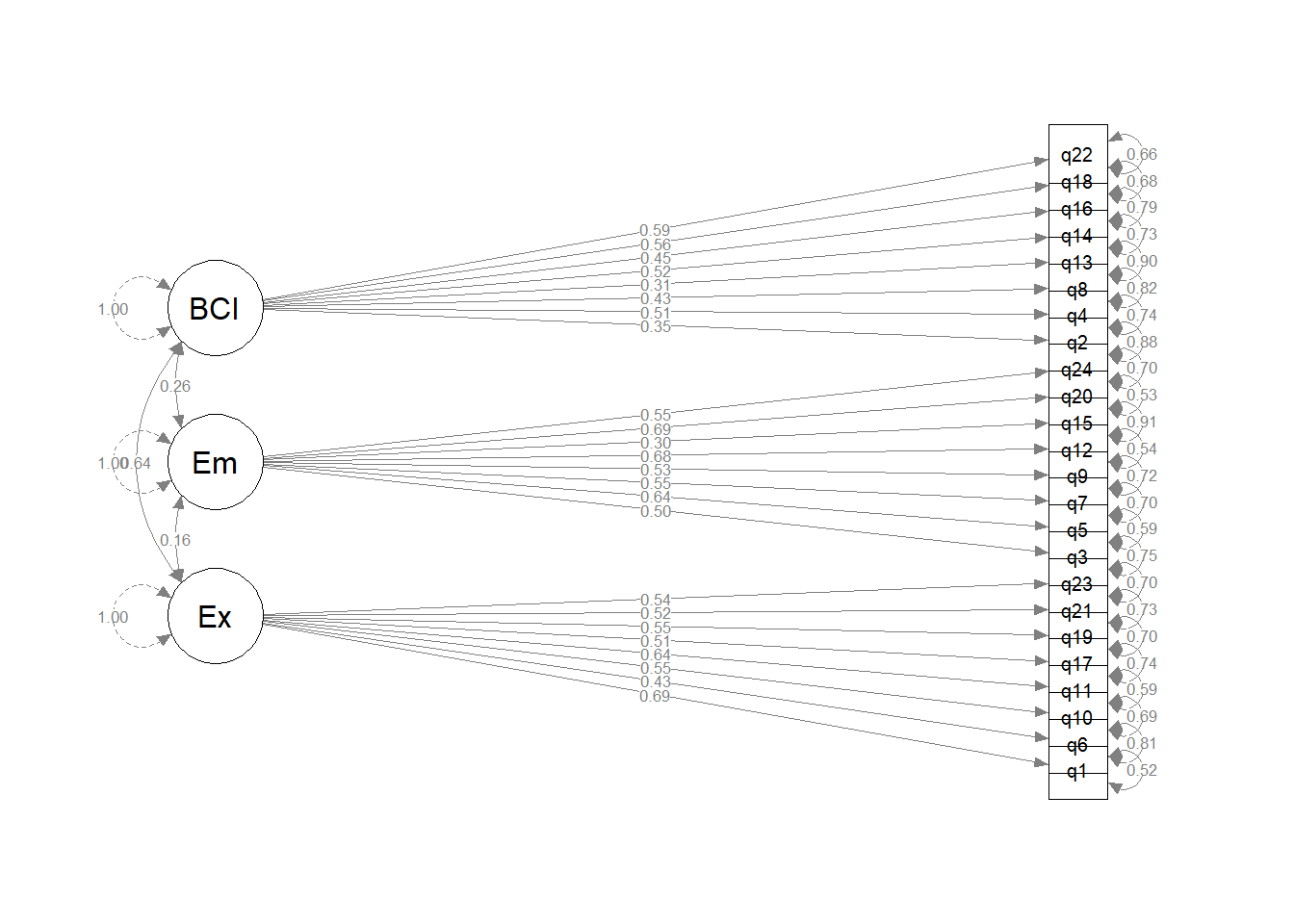
Make a diagram of the model.

Hints

For a quick look at the structure of the model, try the semPaths() function from the semPlot package Chapter 5 CFA#making diagrams.

If you were going to use this sort of diagram in a proper write-up, though, it’d be better to make a nicer graphic manually (e.g., in Powerpoint, your favourite graphics software, or semdiag).

Solution 11. Here’s one example:

library(semPlot)
semPaths(dasmod.est, whatLabels = "std", rotation=2)

There are lots of options in semPaths(), so if you can make your graphic more elaborate than this one, then be our guest!

Optional Question 7

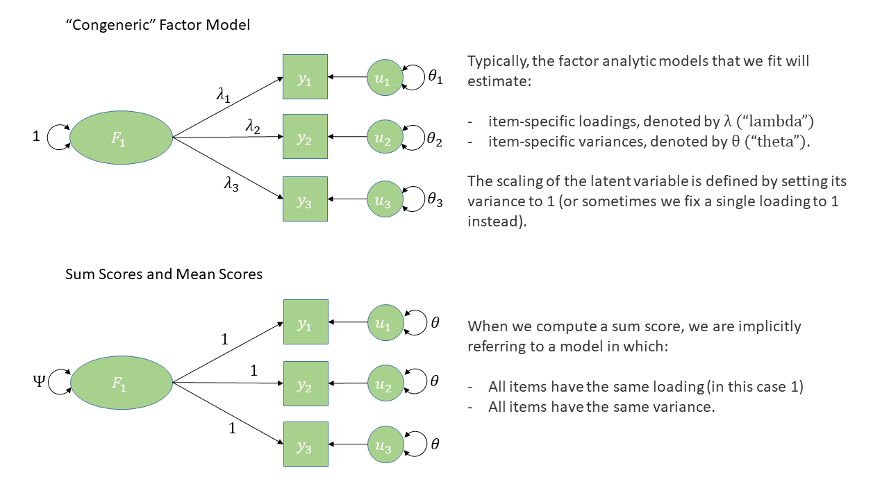
Imagine that you’re a clinician administering the DAS to a patient. In clinical settings, it’s common practice to skip the complex factor analysis we’ve been doing here and just create a sum score or a mean score that describe a patient’s responses. Then clinicians can check whether the score is above some threshold to see whether there’s cause for concern.

For each of the dimensions of apathy in the data, calculate sum scores for each of the 250 participants.

Hints

Good ol’ rowSums() to the rescue!

Solution 12. Here are the sets of items associated with each dimension:

Exitems <- c(1,6,10,11,17,19,21,23)
Emitems <- c(3,5,7,9,12,15,20,24)
BCIitems <- c(2,4,8,13,14,16,18,22)

Again, because the item numbers correspond to the column positions in our data, we can just do rowSums indexing on those column numbers to get our scores:

compl_rdas$ExSCORE <- rowSums(compl_rdas[,Exitems])
compl_rdas$EmSCORE <- rowSums(compl_rdas[,Emitems])
compl_rdas$BCIScore <- rowSums(compl_rdas[,BCIitems])

Optional Question 8

How might you think about a sum/mean score in terms of a diagram?

Hints

What does a sum or mean score imply about how each item is weighted compared to the others? How is this different from what a more sophisticated method like EFA or CFA can do?

Solution 13. Computing sum scores can feel like a ‘model free’ calculation, but actually it does pre-suppose a factor structure, and a much more constrained one than those we have been estimating. Specifically, we’re assuming that all items contribute equally to an underlying factor, rather than being weighted differently, and that all items also have the same variance as one another.

For a full explanation of this idea, see “Thinking twice about sum scores”, McNeish & Wolf 2020.

“DOOM” Scrolling

Dataset: doom.csv

The “Domains of Online Obsession Measure” (DOOM) is a fictitious scale that aims to assess the sub types of addictions to online content. It was developed to measure 2 separate domains of online obsession: items 1 to 9 are representative of the “emotional” relationships people have with their internet usage (i.e. how it makes them feel), and items 10 to 15 reflect “practical” relationship (i.e., how it connects or interferes with their day-to-day life). Each item is measured on a 7-point likert scale from “strongly disagree” to “strongly agree”.

We administered this scale to 476 participants in order to assess the validity of the 2 domain structure of the online obsession measure that we obtained during scale development.

The data are available at https://uoepsy.github.io/data/doom.csv, and the table below shows the individual item wordings.

variable	question
item_1	i just can't stop watching videos of animals
item_2	i spend hours scrolling through tutorials but never actually attempt any projects.
item_3	cats are my main source of entertainment.
item_4	life without the internet would be boring, empty, and joyless
item_5	i try to hide how long i’ve been online
item_6	i avoid thinking about things by scrolling on the internet
item_7	everything i see online is either sad or terrifying
item_8	all the negative stuff online makes me feel better about my own life
item_9	i feel better the more 'likes' i receive
item_10	most of my time online is spent communicating with others
item_11	my work suffers because of the amount of time i spend online
item_12	i spend a lot of time online for work
item_13	i check my emails very regularly
item_14	others in my life complain about the amount of time i spend online
item_15	i neglect household chores to spend more time online

Question 9

Read in the data. It’s all been cleaned already, so we can go straight to modelling.

Assess whether the 2 domain model of online obsession provides a good fit to this validation sample of 476 participants.

Hints

This is essentially asking you to:

1. specify the model
2. estimate the model
3. get some model fit metrics

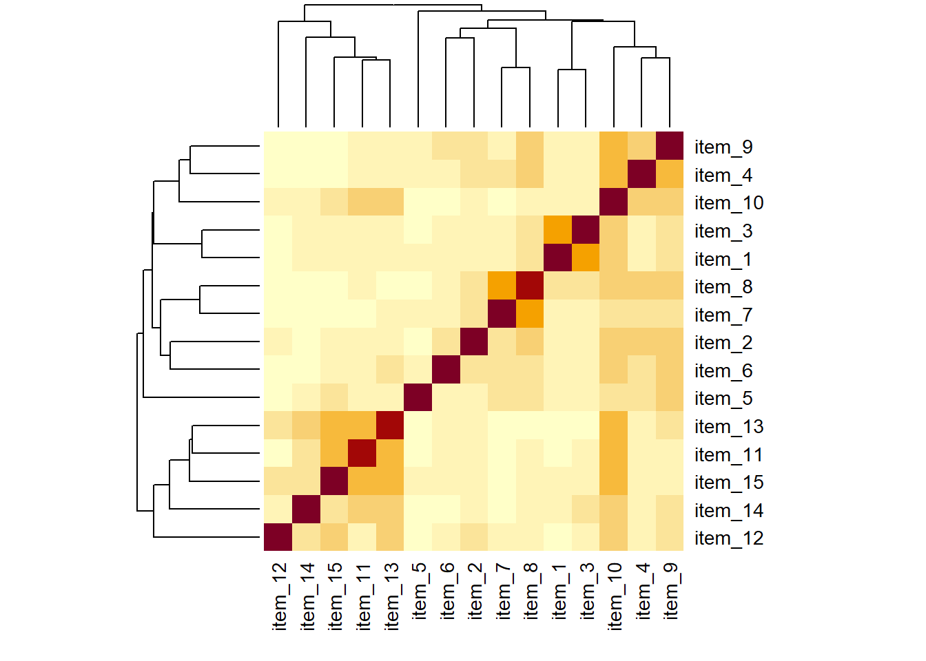
Solution 14. From the visual of the correlation matrix, you can see the vague outline of two groups of items correlations. Note there’s a little overlap..

doom <- read_csv("https://uoepsy.github.io/data/doom.csv")
heatmap(cor(doom))

first we write our model:

moddoom <- "
# emotional domain
emot =~ item_1 + item_2 + item_3 + item_4 + item_5 + item_6 + item_7 + item_8 + item_9
# practical domain
pract =~ item_10 + item_11 + item_13 + item_14 + item_15
# correlated domains (will be estimated by default)
emot ~~ pract
"

Then we fit it to the data:

moddoom.est <- cfa(moddoom, data = doom)

Then we inspect that fitted model object.

Let’s look at the chi-squared test.

summary(moddoom.est)$test$standard

$test
[1] "standard"

$stat
[1] 270

$stat.group
[1] 270

$df
[1] 76

$refdistr
[1] "chisq"

$pvalue
[1] 0

First bad sign: the p-value is so close to zero that it’s just been rounded down to display as 0. This means that the chi-squared test rejects the null hypothesis that the observed covariance matrix is similar to the model-implied covariance matrix. Ideally, we’d want a non-significant p-value here.

OK, let’s extract the fit indices.

fitmeasures(moddoom.est)[c("rmsea","srmr","cfi","tli")]

 rmsea   srmr    cfi    tli 
0.0733 0.0623 0.8479 0.8179 

Uh-oh.. they also don’t look great.

Question 10

Are there any areas of local misfit?

In other words, are there certain parameters that are not in the model (and are therefore fixed to zero) but that could improve model fit if they were estimated?

Hints

Check out the section of Chapter 5 CFA#model-modifications for how to check for little areas of misfit.

Solution 15. I’m printing out just the head(), so that I can look at the few parameters with the greatest modification indices.

modindices(moddoom.est, sort=TRUE) |>
  head()

        lhs op     rhs    mi    epc sepc.lv sepc.all sepc.nox
47   item_1 ~~  item_3 88.70  0.560   0.560    0.459    0.459
32     emot =~ item_10 74.37  1.690   0.817    0.640    0.640
109  item_7 ~~  item_8 61.93  0.370   0.370    0.432    0.432
34     emot =~ item_13 14.82 -0.655  -0.317   -0.275   -0.275
122  item_9 ~~ item_10 12.63  0.145   0.145    0.217    0.217
135 item_13 ~~ item_15  8.96  0.178   0.178    0.171    0.171

The top three parameters jump out immediately to me.

For one: The modification index values are all quite large. These values show how much the model’s chi-squared test statistic would change if we were to include this parameter in the model.

For another, consider the values in the sepc.all column.

• When the operator in the op column is ~~ (that is, when the proposed term is a correlation), then the value in sepc.all can be interpreted like a correlation coefficient. item_1 and item_3 have a suggested correlation of about 0.45, as do item_7 and item_8.

• When the operator is =~ (that is, when the proposed term is a new factor loading), then the value in sepc.all can be interpreted as a standardised factor loading. For emot =~ item_10, a factor loading of 0.6 is worth considering, since it’s well above our threshold for “interestingness” of 0.3.

Question 11

Beware: there’s a slightly blurred line here that we’re about to step over, and move from confirmatory back to ‘exploratory’.

Look carefully at the item wordings. Do any of the suggested modifications make theoretical sense?

Add the top three modifications to the model. Does the new model fit well?

model modifications are exploratory!!

It’s likely you will have to make a couple of modifications in order to obtain a model that fits well to this data.

BUT… we could simply keep adding suggested parameters to our model and we will eventually end up with a perfectly fitting model.

It’s very important to think critically here about why such modifications may be necessary.

• The initial model may have failed to capture the complexity of the underlying relationships among variables. For instance, suggested residual covariances, representing unexplained covariation among observed variables, may indicate misspecification in the initial model.
• The structure of the construct is genuinely different in your population from the initial one in which the scale is developed (this could be a research question in and of itself - i.e. does the structure of “anxiety” differ as people age, or differ between cultures?)

Modifications to a CFA model should be made judiciously, with careful consideration of theory as well as quantitative metrics. The goal is to develop a model that accurately represents the underlying structure of the data while maintaining theoretical coherence and generalizability.

In this case, the likely reason for the poor fit of the “DOOM” scale, is that the person who made the items (ahem, me) doesn’t really know anything about the construct they are talking about, and didn’t put much care into constructing the items!

Solution 16.

variable	question
item_1	i just can't stop watching videos of animals
item_3	cats are my main source of entertainment.
item_7	everything i see online is either sad or terrifying
item_8	all the negative stuff online makes me feel better about my own life
item_10	most of my time online is spent communicating with others

• item_1 ~~ item_3. These questions are both about animals. It would make sense that these are related over and above the underlying “emotional internet usage” factor.
• item_7 ~~ item_8. These are both about viewing negative content online, so it makes sense here that they would be related beyond the ‘emotional’ factor.
• emot =~ item_10. This item is about communicating with others. It currently loads highly on the pract factor too. It maybe makes sense here that “communicating with others” will capture both a practical element of internet usage and an emotional one.

There are three main proposed adjustments from our initial model:

• item_1 ~~ item_3
• item_7 ~~ item_8
• emot =~ item_10

Putting them all in at once could be a mistake. Partly because we want to make the minimal adjustments necessary, and partly because whenever we adjust a model it affects the modification indices, so we should add things one-by-one and re-check modindices() each time. It’s a bit like Whac-A-Mole - you make one modification and then a whole new area of misfits appears!

Let’s adjust our model.
Let’s put the covariance between item_1 and item_3 in. I personally went for this first because they seem more similar to me than item_7 and item_8 do.

moddoom2 <- "
# emotional domain
emot =~ item_1 + item_2 + item_3 + item_4 + item_5 + item_6 + item_7 + item_8 + item_9
# practical domain
pract =~ item_10 + item_11 + item_13 + item_14 + item_15
# correlated domains (will be estimated by default)
emot ~~ pract
item_1 ~~ item_3
"

Then fit it to the data:

moddoom2.est <- cfa(moddoom2, data = doom)

fitmeasures(moddoom2.est)[c("rmsea","srmr","cfi","tli")]

 rmsea   srmr    cfi    tli 
0.0536 0.0519 0.9199 0.9028 

The fit is still not great, but it’s better (it was always going to be!). And the other suggested correlations are still present in modification indices:

modindices(moddoom2.est, sort=TRUE) |>
  head()

       lhs op     rhs    mi    epc sepc.lv sepc.all sepc.nox
33    emot =~ item_10 73.22  1.941   0.804    0.630    0.630
109 item_7 ~~  item_8 61.52  0.371   0.371    0.437    0.437
35    emot =~ item_13 13.53 -0.728  -0.301   -0.261   -0.261
122 item_9 ~~ item_10 12.87  0.147   0.147    0.220    0.220
44   pract =~  item_7  8.76 -0.246  -0.240   -0.215   -0.215
87  item_4 ~~ item_10  8.62  0.139   0.139    0.174    0.174

Let’s add both of those other correlations into the model and fit it:

moddoom3 <- "
# emotional domain
emot =~ item_1 + item_2 + item_3 + item_4 + item_5 + item_6 + item_7 + item_8 + item_9
# practical domain
pract =~ item_10 + item_11 + item_13 + item_14 + item_15
# correlated domains (will be estimated by default)
emot ~~ pract
item_1 ~~ item_3
item_7 ~~ item_8
"

moddoom3.est <- cfa(moddoom3, data = doom)

fitmeasures(moddoom3.est)[c("rmsea","srmr","cfi","tli")]

 rmsea   srmr    cfi    tli 
0.0354 0.0443 0.9654 0.9575 

Whoop! It fits well! It may well be that if we inspect modification indices again, we still see that emot =~ item_10 would improve our model fit. I’m more reluctant to include that one as doing so will change slightly the meaning of our latent factor emot. So it becomes much harder to defend that we are testing the same theoretical model.

The other thing to remember is that we could simply keep adding parameters until we run out of degrees of freedom, and our model would “fit better”. But such a model would not be useful. It would not generalise well, becaue it runs the risk of being overfitted to the nuances of this specific sample.