W2 Exercises: Introducing MLM

MLM Demonstration

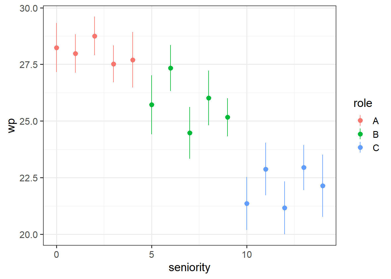
These first set of exercises are not “how to do analyses with multilevel models” - they are designed to get you thinking, and help with an understanding of how these models work.

Question 1

Recall the data from last week’s exercises. Instead of looking at the roles A, B and C, we’ll look in more fine grained detail at the seniority. This is mainly so that we have a continuous variable to work with as it makes this illustration easier.

The chunk of code below shows a function for plotting that you might not be familiar with - stat_summary(). This takes the data in the plot and “summarises” the Y-axis variable into the mean at every unique value on the x-axis. So below, rather than having a lot of individual data points that represent every employee’s wp (workplace pride), we let stat_summary() compute the mean (the points) plus and minus the standard error (the vertical lines) of all the wp observations at each value of seniority:

library(tidyverse)
jsup <- read_csv("https://uoepsy.github.io/data/lmm_jsup.csv")

ggplot(jsup, aes(x = seniority, y = wp, col = role)) +
  stat_summary(geom="pointrange")

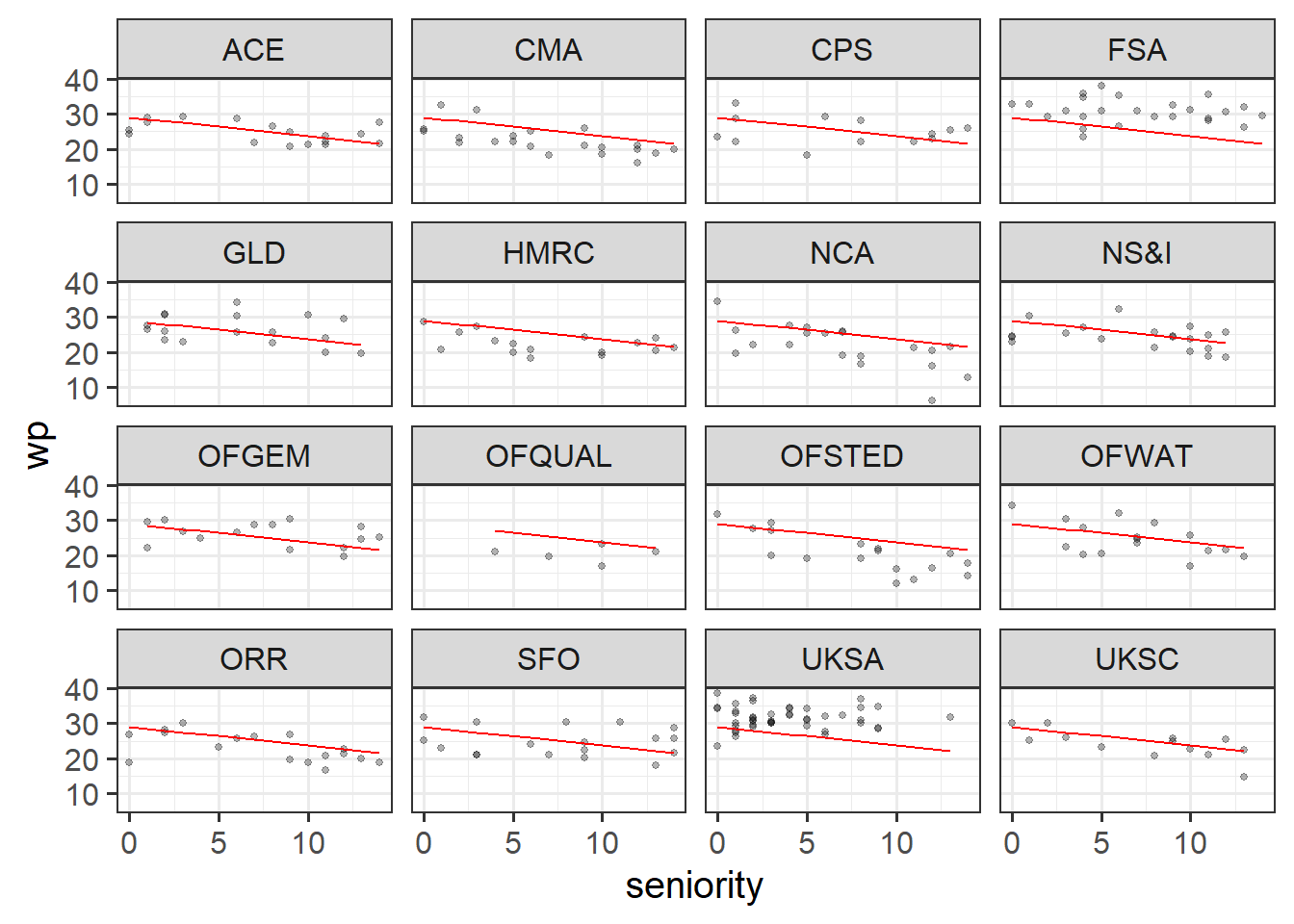
Below is some code that fits a model of the workplace-pride predicted by seniority level. Line 2 then gets the ‘fitted’ values from the model and adds them as a new column to the dataset, called pred_lm. The fitted values are what the model predicts the workplace pride to be for every value of seniority.

Lines 4-7 then plot the data, split up by each department, and adds lines showing the model fitted values.

Run the code and check that you get a plot. What do you notice about the lines?

lm_mod <- lm(wp ~ seniority, data = jsup)
jsup$pred_lm <- predict(lm_mod)

ggplot(jsup, aes(x = seniority)) + 
  geom_point(aes(y = wp), size=1, alpha=.3) +
  facet_wrap(~dept) +
  geom_line(aes(y=pred_lm), col = "red")

Solution 1. We should get something like this:

lm_mod <- lm(wp ~ seniority, data = jsup)
jsup$pred_lm <- predict(lm_mod)

ggplot(jsup, aes(x = seniority)) + 
  geom_point(aes(y = wp), size=1, alpha=.3) +
  facet_wrap(~dept) +
  geom_line(aes(y=pred_lm), col = "red")

Note that the lines are exactly the same for each department. This makes total sense, because the model (which is where we’ve got the lines from) completely ignores the department variable!

Question 2

Below are 3 more code chunks that all 1) fit a model, then 2) add the fitted values of that model to the plot.

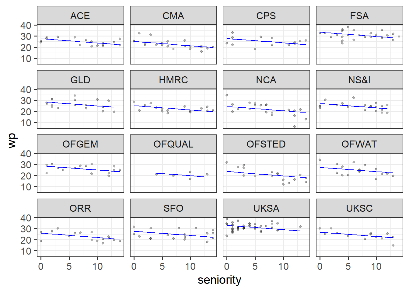
The first model is a ‘no-pooling’ approach, similar to what we did in last week’s exercises - adding in dept as a predictor.

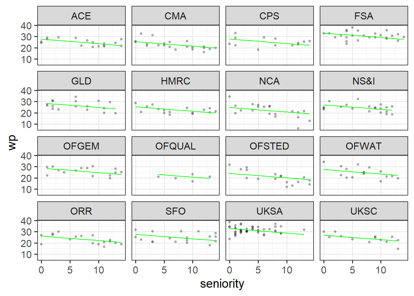
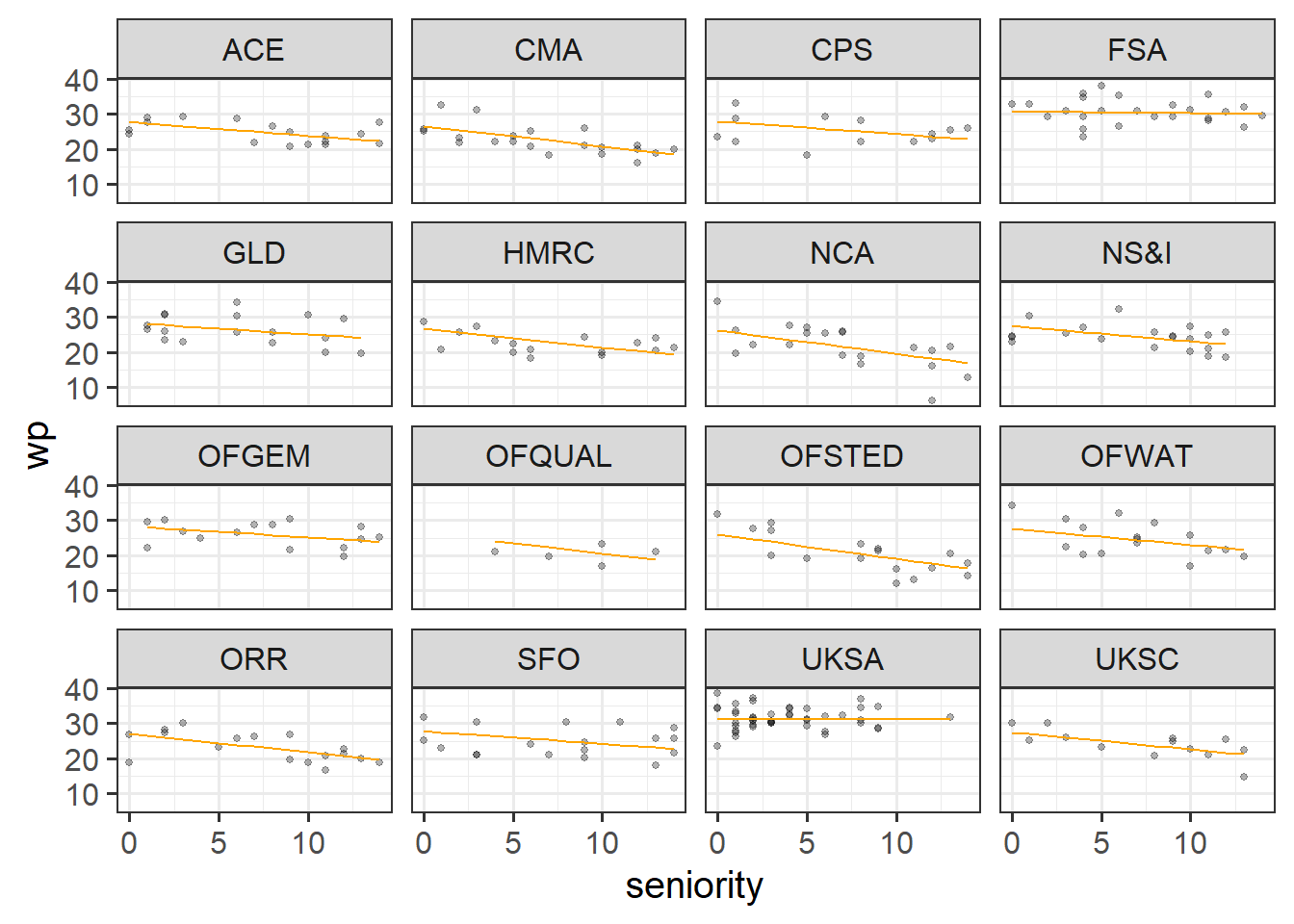
The second and third are multilevel models. The second fits random intercepts by-department, and the third fits random intercepts and slopes of seniority.

Copy each chunk and run through the code. Pay attention to how the lines differ.

fe_mod <- lm(wp ~ dept + seniority, data = jsup)
jsup$pred_fe <- predict(fe_mod)

ggplot(jsup, aes(x = seniority)) + 
  geom_point(aes(y = wp), size=1, alpha=.3) +
  facet_wrap(~dept) +
  geom_line(aes(y=pred_fe), col = "blue")

library(lme4)
ri_mod <- lmer(wp ~ seniority + (1|dept), data = jsup)
jsup$pred_ri <- predict(ri_mod)

ggplot(jsup, aes(x = seniority)) + 
  geom_point(aes(y = wp), size=1, alpha=.3) +
  facet_wrap(~dept) +
  geom_line(aes(y=pred_ri), col = "green")

rs_mod <- lmer(wp ~ seniority + (1 + seniority|dept), data = jsup)
jsup$pred_rs <- predict(rs_mod)

ggplot(jsup, aes(x = seniority)) + 
  geom_point(aes(y = wp), size=1, alpha=.3) +
  facet_wrap(~dept) +
  geom_line(aes(y=pred_rs), col = "orange")

Solution 2. With the first model, wp ~ seniority + dept, we are saying the following things:

• We allow the model to estimate an association between workplace pride and seniority. This line is estimated without respect to department, or in other words, for the “average” department.
• We also allow the model to take that line and shift it up and down for each different department. The slope of the line stays the same. All that’s changing is the vertical position of the line.
  • Look at UKSA and FSA: the lines are shifted up compared to the others.
  • Look at UKSC and OFSTED: the lines are shifted down compared to the others.

fe_mod <- lm(wp ~ dept + seniority, data = jsup)
jsup$pred_fe <- predict(fe_mod)

ggplot(jsup, aes(x = seniority)) + 
  geom_point(aes(y = wp), size=1, alpha=.3) +
  facet_wrap(~dept) +
  geom_line(aes(y=pred_fe), col = "blue")

With the second model, wp ~ seniority + (1|dept), we are saying the following things:

• We allow the model to estimate an association between workplace pride and seniority.
• With (1|dept), we allow the model to adjust the intercept of that line, depending on the scores of each department.
  • In other words, the wp ~ seniority bit is modelling the average line for all departments, and the (1|dept) bit is saying “now nudge that line up or down so that it fits the data of each individual department better”.
  • This is very similar to the fixed-effects-based model above. The difference is that the nudges up and down are now drawn from a single distribution, so they are all slightly closer to the mean of departments than the changes that the model above made.
  • People often call these “random intercepts by department”. You may also hear “intercept adjustments by department”.
  • If we look at this model’s summary, we can see how it combines all these individual adjustments into a distribution and give us some summary statistics. This way, we can see how big the adjustments tend to be.

Side note: Why use random effects instead of fixed effects, if they do the same thing?

• They don’t really do the same thing: random effects can also include random slopes, which the fixed-effect model cannot do. We’ll see random slopes next.
• Fixed effects are generally used for predictors that we have particular hypotheses/predictions about. Random effects are used when we have other sources of non-independence we need to tell the model about.

library(lme4)
ri_mod <- lmer(wp ~ seniority + (1|dept), data = jsup)
jsup$pred_ri <- predict(ri_mod)

ggplot(jsup, aes(x = seniority)) + 
  geom_point(aes(y = wp), size=1, alpha=.3) +
  facet_wrap(~dept) +
  geom_line(aes(y=pred_ri), col = "green")

Finally, with the third model, wp ~ seniority + (1 + seniority|dept), we are saying the following things:

• We allow the model to estimate an association between workplace pride and seniority, for departments on average. That’s the wp ~ seniority bit, like before.
• With (1 + seniority|dept), we allow the model to adjust the intercept of that line AND to adjust the slope of that line for each individual department.
  • In other words, the wp ~ seniority bit is modelling the average line for all departments, and the (1 + seniority|dept) bit is saying “now nudge that line up or down AND change how steep it is, so that it fits the data of each individual department better”.
  • People often call these “random intercepts by department and random slopes over seniority by department”. You may also hear “intercept adjustments by department and adjustments to the slope of seniority by department”.
  • If we look at this model’s summary, we can see how it combines all these individual adjustments into a distribution of intercept adjustments and a distribution of slope adjustments, and give us some summary statistics about both. This way, we can see how big the adjustments tend to be.

So in this next plot, the height of the lines is changing, but additionally, each department’s association between seniority and workplace pride can be different. Some departments (OFQUAL, OFSTED, ORR) have a negative association, some have a flatter association (e.g, FSA, UKSA etc).

rs_mod <- lmer(wp ~ seniority + (1 + seniority|dept), data = jsup)
jsup$pred_rs <- predict(rs_mod)

ggplot(jsup, aes(x = seniority)) + 
  geom_point(aes(y = wp), size=1, alpha=.3) +
  facet_wrap(~dept) +
  geom_line(aes(y=pred_rs), col = "orange")

Question 3

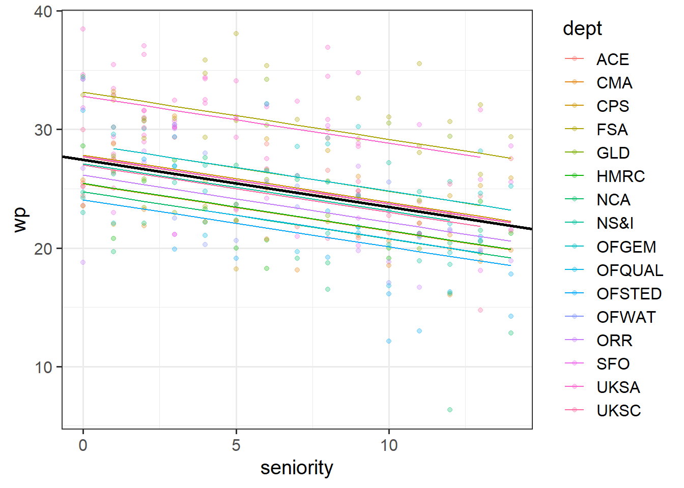
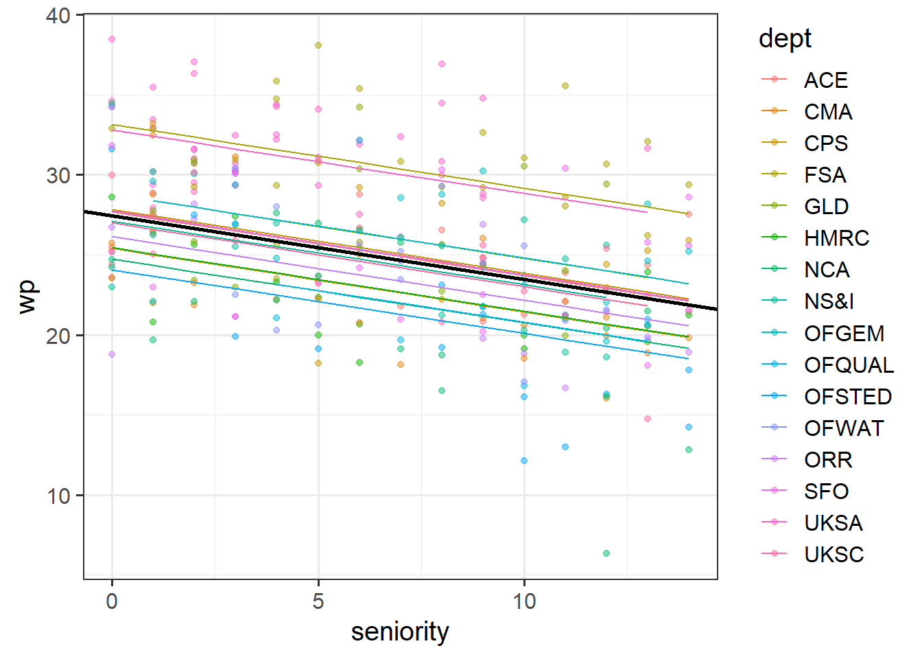
From the previous questions you should have a model called ri_mod.

Below is a plot of the fitted values from that model. Rather than having a separate facet for each department as we did above, I have put them all on one plot. The thick black line is the average intercept and slope of the departments lines.

Identify the parts of the plot that correspond to A1-4 in the summary output of the model below

Hints

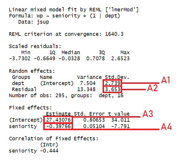
Choose from these options:

• where the black line cuts the y axis (at x=0)
  
• the slope of the black line
  
• the standard deviation of the distances from all the individual datapoints (employees) to the line for the department in which it works.
  
• the standard deviation of the distances from all the individual department lines to the black line

Solution 3.

• A1 = the standard deviation of the distances from all the individual department lines to the black line
  
• A2 = the standard deviation of the distances from all the individual datapoints (employees) to the line for the department in which it works.
• A3 = where the black line cuts the y axis
  
• A4 = the slope of the black line

Optional Extra

Below is the model equation for the ri_mod model.

Identify the part of the equation that represents each of A1-4.

\[\begin{align} \text{For Employee }j\text{ from Dept }i & \\ \text{Level 1 (Employee):}& \\ \text{wp}_{ij} &= b_{0i} + b_1 \cdot \text{seniority}_{ij} + \epsilon_{ij} \\ \text{Level 2 (Dept):}& \\ b_{0i} &= \gamma_{00} + \zeta_{0i} \\ \text{Where:}& \\ \zeta_{0i} &\sim N(0,\sigma_{0}) \\ \varepsilon &\sim N(0,\sigma_{e}) \\ \end{align}\]

Hints

Choose from:

• \(\sigma_{\varepsilon}\)
  
• \(b_{1}\)
  
• \(\sigma_{0}\)
  
• \(\gamma_{00}\)

Solution 4.

• A1 = \(\sigma_{0}\)
  
• A2 = \(\sigma_{\varepsilon}\)
  
• A3 = \(\gamma_{00}\)
  
• A4 = \(b_{1}\)

Audio Interference in Executive Functioning (Repeated Measures)

This next set are a bit closer to conducting a real study. We have some data and a research question (below). The exercises will walk you through describing the data, then prompt you to think about how we might fit an appropriate model to address the research question, and finally task you with having a go at writing up what you’ve done.

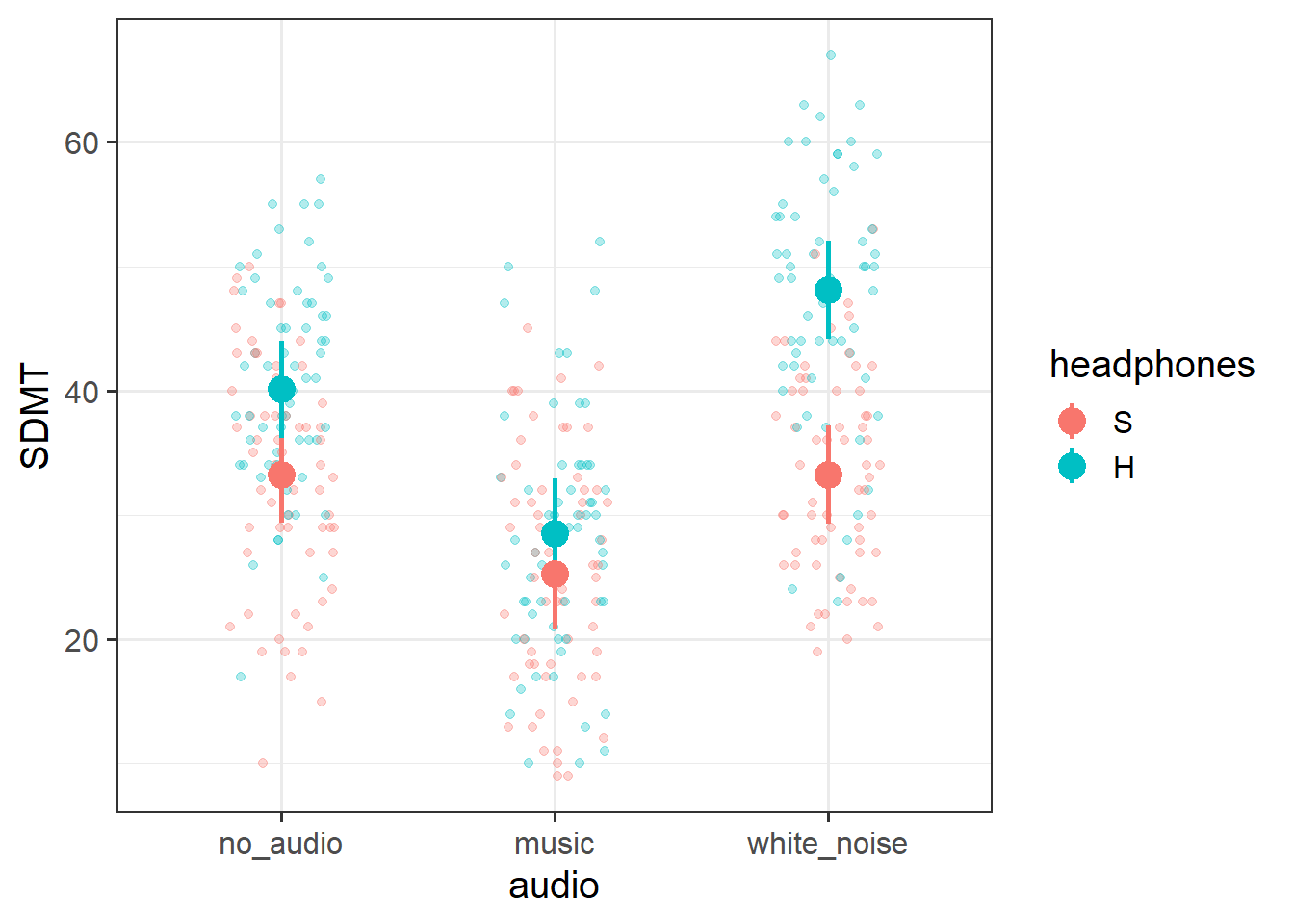
Data: Audio interference in executive functioning

This data is from a simulated study that aims to investigate the following research question:

How do different types of audio interfere with executive functioning, and does this interference differ depending upon whether or not noise-cancelling headphones are used?

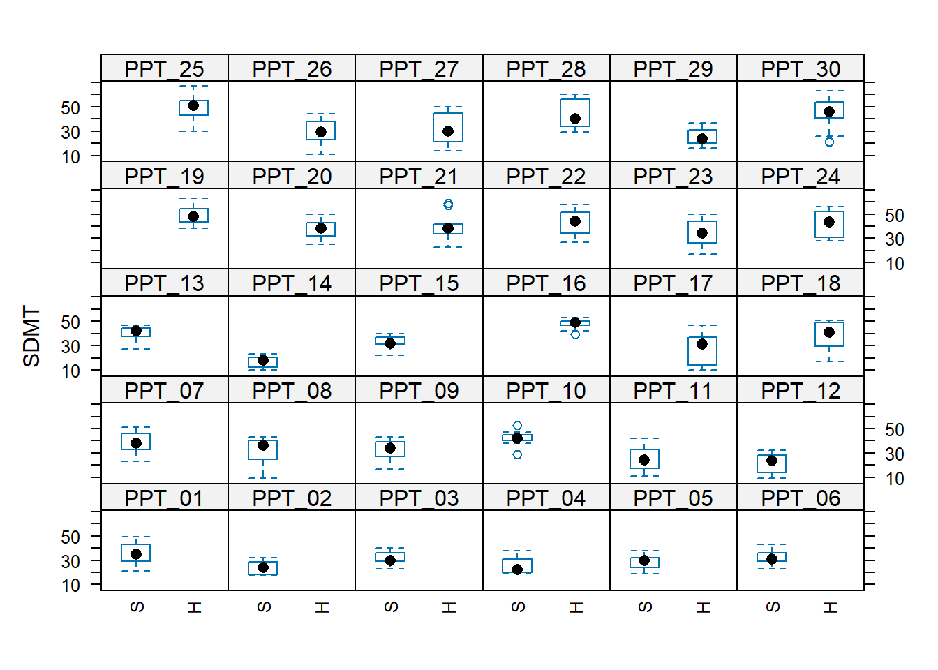
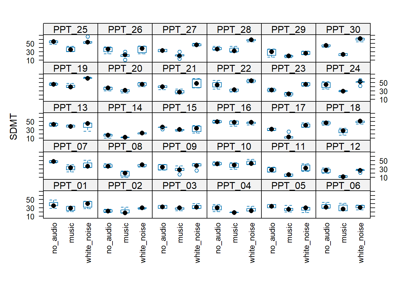
30 healthy volunteers each completed the Symbol Digit Modalities Test (SDMT) - a commonly used test to assess processing speed and motor speed - a total of 15 times. During the tests, participants listened to either no audio (5 tests), white noise (5 tests) or classical music (5 tests). Half the participants listened via active-noise-cancelling headphones, and the other half listened via speakers in the room. Unfortunately, lots of the tests were not administered correctly, and so not every participant has the full 15 trials worth of data.

The data is available at https://uoepsy.github.io/data/lmm_ef_sdmt.csv.

variable	description
PID	Participant ID
audio	Audio heard during the test ('no_audio', 'white_noise','music')
headphones	Whether the participant listened via speakers (S) in the room or via noise cancelling headphones (H)
SDMT	Symbol Digit Modalities Test (SDMT) score

Question 4

How many participants are there in the data?
How many have complete data (15 trials)?
What is the average number of trials that participants completed? What is the minimum?
Does every participant have some data for each type of audio?

Hints

Functions like table() and count() will likely be useful here.

Solution 5.

efdat <- read_csv("https://uoepsy.github.io/data/lmm_ef_sdmt.csv")
head(efdat)

# A tibble: 6 × 4
  PID    audio       headphones  SDMT
  <chr>  <chr>       <chr>      <dbl>
1 PPT_15 no_audio    S             37
2 PPT_22 no_audio    H             55
3 PPT_21 no_audio    H             40
4 PPT_20 no_audio    H             36
5 PPT_20 no_audio    H             30
6 PPT_05 white_noise S             30

Solution 6. For a quick “how many?”, functions like n_distinct() can be handy:

n_distinct(efdat$PID)

[1] 30

Which is essentially the same as asking:

unique(efdat$PID) |> length()

[1] 30

Solution 7. Here are the counts of trials for each participant.

efdat |> 
  count(PID)

# A tibble: 30 × 2
  PID        n
  <chr>  <int>
1 PPT_01    13
2 PPT_02    12
3 PPT_03    10
4 PPT_04    10
5 PPT_05    10
# ℹ 25 more rows

We can pass that to something like summary() to get a quick descriptive of the n column, and so we can see that no participant completed all 15 trials (max is 14). Everyone completed at least 10, and the median was 12.

efdat |> 
  count(PID) |>
  summary()

     PID                  n     
 Length:30          Min.   :10  
 Class :character   1st Qu.:11  
 Mode  :character   Median :12  
                    Mean   :12  
                    3rd Qu.:13  
                    Max.   :14  

We could also do this easily with things like:

table(efdat$PID) |> median()

[1] 12

Solution 8. For this kind of thing I would typically default to using table() for smaller datasets, to see how many datapoints are in each combination of PID and audio:

table(efdat$PID, efdat$audio)

        
         music no_audio white_noise
  PPT_01     4        5           4
  PPT_02     5        4           3
  PPT_03     3        2           5
  PPT_04     3        4           3
  PPT_05     5        2           3
  PPT_06     4        4           5
  PPT_07     4        3           4
  PPT_08     4        4           5
  PPT_09     5        4           5
  PPT_10     4        5           4
  PPT_11     4        4           4
  PPT_12     4        5           5
  PPT_13     4        4           3
  PPT_14     3        5           4
  PPT_15     4        5           4
  PPT_16     4        4           3
  PPT_17     5        4           5
  PPT_18     5        3           3
  PPT_19     3        5           3
  PPT_20     4        4           5
  PPT_21     3        5           4
  PPT_22     4        4           3
  PPT_23     3        3           4
  PPT_24     4        5           5
  PPT_25     4        4           5
  PPT_26     5        4           5
  PPT_27     5        2           4
  PPT_28     4        4           4
  PPT_29     4        4           4
  PPT_30     2        5           3

From the above, we can see that everyone has data from \(\geq 2\) trials for a given audio type.

table(efdat$PID, efdat$audio) |> min()

[1] 2

a tidyverse way:

When tables get too big, we can do the same thing with count(), but we need to make sure that we are working with factors, in order to summarise all possible combinations of groups (even empty ones)

efdat |> 
  mutate(PID = factor(PID),
         audio = factor(audio)) |>
  # the .drop=FALSE means "keep empty groups"
  count(PID,audio,.drop=FALSE) |> 
  summary()

      PID             audio          n    
 PPT_01 : 3   music      :30   Min.   :2  
 PPT_02 : 3   no_audio   :30   1st Qu.:4  
 PPT_03 : 3   white_noise:30   Median :4  
 PPT_04 : 3                    Mean   :4  
 PPT_05 : 3                    3rd Qu.:5  
 PPT_06 : 3                    Max.   :5  
 (Other):72                               

There are plenty of other ways (e.g., you could use combinations of group_by(), summarise()), so just pick one that makes sense to you.

Question 5

How do different types of audio interfere with executive functioning, and does this interference differ depending upon whether or not noise-cancelling headphones are used?

Consider the following questions about the study:

• What is our outcome of interest?
  
• What variables are we seeking to investigate in terms of their impact on the outcome?
  
• What does a row of data represent?
• Are the rows of data clustered/grouped? In what way?
  
• What varies within these clusters?
• What varies between these clusters?

Solution 9.

• What is our outcome of interest?
  • SDMT scores
    
• What variables are we seeking to investigate in terms of their impact on the outcome?
  • audio type and the interaction audio type \(\times\) wearing headphones
• What does a row of data represent?
  • individual trials
    
• Are the rows of data grouped/clustered? In what way?
  • participants
    
• What varies within these clusters?
  • the type of audio
    
• What varies between these clusters?
  • whether they listen via headphones or speakers

Question 6

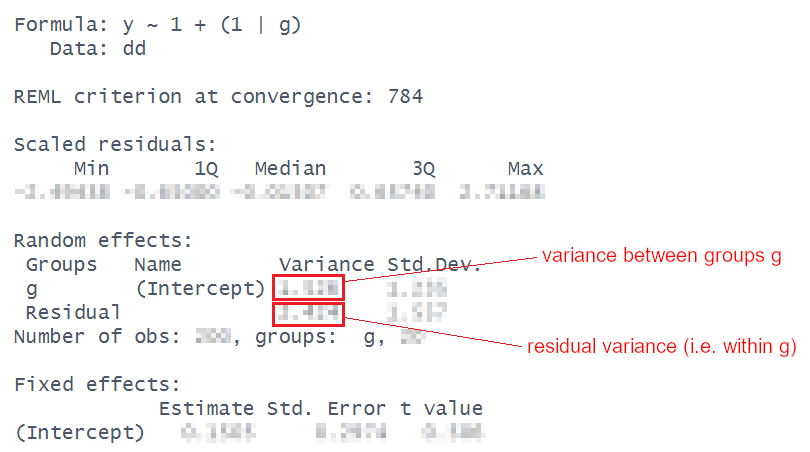
A model that only has an intercept, i.e., y ~ 1, is called an “intercept-only model”. A multilevel model that only has an intercept but also has a grouping structure, i.e., y ~ 1 + (1|g) is called an “intercept-only model with random intercepts”. (Here g stands for an arbitrary group.)

Because there are no predictors in the fixed effects, the model only estimates one fixed parameter: the intercept. All of the variance in the outcome gets modelled in the random effects part, and is partitioned into either ‘variance between groups’ or ‘residual variance’. This means we can just use those estimates to calculate the ICC (the Intraclass Correlation Coefficient).

For our executive functioning study, fit an intercept-only model with random intercepts for the appropriate outcome variable and the appropriate grouping variable (check your responses to the last question to remind yourself what these variables are for this dataset). Use the output to calculate the ICC. Compare it to the answer you get from ICCbare() (it should be pretty close).

Hints

The formula for the ICC is:
\[ ICC = \frac{\sigma^2_{b}}{\sigma^2_{b} + \sigma^2_e} = \frac{\text{between-group variance}}{\text{between-group variance}+\text{within-group variance}} \]

Solution 10.

nullmod <- lmer(SDMT ~ 1 + (1 | PID), data = efdat)
summary(nullmod)

Linear mixed model fit by REML ['lmerMod']
Formula: SDMT ~ 1 + (1 | PID)
   Data: efdat

REML criterion at convergence: 2665

Scaled residuals: 
    Min      1Q  Median      3Q     Max 
-2.5868 -0.6826  0.0324  0.6570  2.2674 

Random effects:
 Groups   Name        Variance Std.Dev.
 PID      (Intercept) 62.0     7.88    
 Residual             79.8     8.93    
Number of obs: 360, groups:  PID, 30

Fixed effects:
            Estimate Std. Error t value
(Intercept)    34.79       1.51      23

\(\frac{62.02}{62.02+79.82} = 0.44\), or 44% of the variance in SDMT scores is explained by participant differences.

This matches (closely enough) with the ICCbare() function:

library(ICC)
ICCbare(x = PID, y = SDMT, data = efdat)

[1] 0.436

Question 7

Make factors and set the reference levels of the audio and headphones variables to “no audio” (no_audio) and “speakers” (S) respectively.

Hints

Can’t remember about setting factors and reference levels? Check back to DAPR2!

Solution 11.

efdat <- efdat %>%
  mutate(
    audio = fct_relevel(factor(audio), "no_audio"),
    headphones = fct_relevel(factor(headphones), "S")
  )

Question 8

Fit a multilevel model to address the aims of the study (copied below)

How do different types of audio interfere with executive functioning, and does this interference differ depending upon whether or not noise-cancelling headphones are used?

Specifying the model may feel like a lot, but try splitting it into three parts:

\[ \text{lmer(}\overbrace{\text{outcome }\sim\text{ fixed effects}}^1\, + \, (1 + \underbrace{\text{slopes}}_3\, |\, \overbrace{\text{grouping structure}}^2 ) \]

1. Just like the lm()s we have used in the past, think about what we want to test. This should provide the outcome and the structure of our fixed effects.
   
2. Think about how the observations are clustered/grouped. This should tell us how to specify the grouping structure in the random effects.
   
3. Some conditions are within-group (i.e., every member of the group contributes to every condition), some conditions are between-group (i.e., every member of the group contributes to only one condition). You can only use random slopes for within-group conditions. Think about what variable(s) you have within-group data for. This provides you with what to put in as random slopes.

Hints

Make sure to read about multilevel models and how to fit them in 2: MLM #multilevel-models-in-r.

Solution 12. The question
    “How do different types of audio interfere with executive functioning” means we are interested in the effects of audio type (audio) on executive functioning (SDMT scores), so we will want:

lmer(SDMT ~ audio ...

However, the research aim also asks
    “… and does this interference differ depending upon whether or not noise-cancelling headphones are used?”
which suggests that we are interested in the interaction SDMT ~ audio * headphones

lmer(SDMT ~ audio * headphones + ...   

Solution 13. There are lots of ways that our data is grouped.
We have:

• 3 different groups of audio type (no_audio, white_noise, music)
• 2 groups of listening condition (S, H)
• 30 groups of participants (“PPT_01”, “PPT_02”, “PPT_03”, …)

The effects of audio type and headphones are both things we actually want to test - these variables are in our fixed effects. The levels of audio and headphones are not just a random sample from a wider population of levels - they’re a specific set of things we want to compare SDMT scores between.

Compare this with the participants - we don’t care about if there is a difference in SDMT scores between e.g., “PPT_03” and “PPT_28”. The participants themselves are just a sample of people that we have taken from a wider population. This makes thinking of “by-participant random effects” a sensible approach - we model differences between participants as a normal distribution of deviations around some average:

lmer(SDMT ~ audio * headphones + (1 + ... | PID)  

The minimum that we can include is the random intercept. What (1|PID) specifies is that “participants vary in their SDMT scores”. This makes sense - we would expect some participants to have higher executive functioning (and so will tend to score high on the SDMT), and others to have lower functioning (and so tend to score lower).

Solution 14. We can also include a random by-participant effect of audio.
audio|PID specifies that the effect of audio type on SDMT varies by participant. This seems feasible - music might be very distracting (and interfere a lot with the test) for some participants, but have a negligible effect for others.

lmer(SDMT ~ audio * headphones + 
              (1 + audio | PID), data = efdat)

Why can’t we have (headphones|PID)?

Why can we fit (1 + audio | PID) but not (1 + headphones | PID), or both (1 + audio + headphones | PID) or (1 + audio * headphones | PID)?

Remember that y ~ ... + (x | g) is saying “the slope of y~x varies by g”.
Such a sentence only makes sense if each “the slope of y~x” is defined for every (or most) groups.

For the headphones predictor, every participant is either in the “S” (speakers) condition or the “H” (headphones) condition.
This means that “the effect of headphones on SDMT” doesn’t exist for any single participant! This means it makes no sense to try and think of the effect as ‘varying by participant’.

Compare this to the audio predictor, for the effect does exist for a single given participant, therefore it is possible to think of it as being different for different participants (e.g. PPT_30’s performance improves with white noise, but PPT_16’s performance does not).

The plots below may help to cement this idea:

Question 9

We now have a model, but we don’t have any p-values or confidence intervals or anything - i.e. we have no inferential criteria on which to draw conclusions. There are a whole load of different methods available for drawing inferences from multilevel models, which means it can be a bit of a never-ending rabbit hole. For now, we’ll just use the ‘quick and easy’ approach provided by the lmerTest package seen in the lectures.

Using the lmerTest package, re-fit your model, and you should now get some p-values!

Hints

If you use library(lmerTest) to load the package, then every single model you fit will show p-values calculated with the Satterthwaite method.
Personally, I would rather this is not the case, so I often opt to fit specific models with these p-values without ever loading the package:
modp <- lmerTest::lmer(y ~ 1 + x + ....

optional: a model comparison

If we want to go down the model comparison route, we just need to isolate the relevant part(s) of the model that we are interested in.

Remember, model comparison is sometimes a useful way of testing a set of coefficients. For instance, in this example the interaction involves estimating two terms: audiomusic:headphonesH and audiowhite_noise:headphonesH.

To test the interaction as a whole, we can create a model without the interaction, and then compare it. The SATmodcomp() function from the pbkrtest package provides a way of conducting an F test with the same Satterthwaite method of approximating the degrees of freedom:

sdmt_mod <- lmer(SDMT ~ audio * headphones + 
              (1 + audio | PID), data = efdat)
sdmt_res <- lmer(SDMT ~ audio + headphones + 
                   (1 + audio | PID), data = efdat)
library(pbkrtest)
SATmodcomp(largeModel = sdmt_mod, smallModel = sdmt_res)

large : SDMT ~ audio * headphones + (1 + audio | PID)
small : SDMT ~ audio + headphones + (1 + audio | PID)
     statistic  ndf  ddf p.value    
[1,]      11.1  2.0 26.9 0.00031 ***
---
Signif. codes:  0 '***' 0.001 '**' 0.01 '*' 0.05 '.' 0.1 ' ' 1

Solution 15.

sdmt_mod <- lmerTest::lmer(SDMT ~ audio * headphones + 
              (1 + audio | PID), data = efdat)

summary(sdmt_mod)

Linear mixed model fit by REML. t-tests use Satterthwaite's method [
lmerModLmerTest]
Formula: SDMT ~ audio * headphones + (1 + audio | PID)
   Data: efdat

REML criterion at convergence: 2376

Scaled residuals: 
    Min      1Q  Median      3Q     Max 
-2.3452 -0.6286  0.0576  0.6081  2.2125 

Random effects:
 Groups   Name             Variance Std.Dev. Corr       
 PID      (Intercept)      51.2     7.15                
          audiomusic       13.7     3.70      0.03      
          audiowhite_noise 15.2     3.90     -0.25 -0.16
 Residual                  31.5     5.61                
Number of obs: 360, groups:  PID, 30

Fixed effects:
                             Estimate Std. Error      df t value Pr(>|t|)    
(Intercept)                   33.2580     1.9890 28.2206   16.72  3.5e-16 ***
audiomusic                    -8.0173     1.4115 27.5877   -5.68  4.6e-06 ***
audiowhite_noise              -0.0304     1.4450 26.3259   -0.02  0.98335    
headphonesH                    6.8531     2.8117 28.1923    2.44  0.02135 *  
audiomusic:headphonesH        -3.5875     2.0013 27.9401   -1.79  0.08388 .  
audiowhite_noise:headphonesH   8.0246     2.0450 26.4617    3.92  0.00056 ***
---
Signif. codes:  0 '***' 0.001 '**' 0.01 '*' 0.05 '.' 0.1 ' ' 1

Correlation of Fixed Effects:
            (Intr) audmsc adwht_ hdphnH adms:H
audiomusic  -0.174                            
audiowht_ns -0.352  0.192                     
headphonesH -0.707  0.123  0.249              
admsc:hdphH  0.123 -0.705 -0.135 -0.173       
adwht_ns:hH  0.249 -0.136 -0.707 -0.351  0.191

Question 10

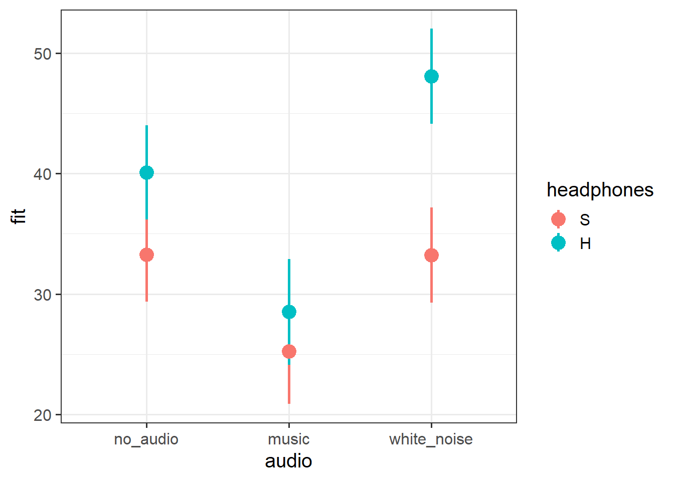
We’ve already seen in the example with the UK civil service employees (above and last week) that we can visualise the fitted values (model predictions). But these were plotting all the cluster-specific values, and what we are typically really interested in are the estimates of (and uncertainty around) our fixed effects (i.e. estimates for clusters on average). We say “typically” because if you study individual differences, for example, sometimes you might really care about estimating the variability within and between people! But for now, we’re going to focus on what most research questions target: the fixed effects.

Using tools like the effects package can provide us with the values of the outcome across levels of a specific fixed predictor (holding other predictors at their mean).

Your task is to make a plot that visualises the model’s fixed effect estimates.

This should get you started:

library(effects)
effect(term = "audio*headphones", mod = sdmt_mod) |>
  as.data.frame()

Hints

You can see the effects package used for plotting in 2: MLM #visualising-models.
(You’ll have to use different geoms than this example does because the example involves a continuous and a categorical predictor, whereas this data set has two categorical ones.)

Solution 16.

library(effects)
effect(term = "audio*headphones", mod = sdmt_mod) |>
  as.data.frame() |>
  ggplot(aes(x=audio,y=fit,
             ymin=lower,ymax=upper,
             col=headphones))+
  geom_pointrange(size=1,lwd=1)

Question 11

Now we have some p-values and a plot, try to create a short write-up of the analysis and results.

Hints

Think about the principles that have guided you during write-ups thus far.

The aim in writing a statistical report should be that a reader is able to more or less replicate your analyses without referring to your analysis code. Furthermore, it should be able for a reader to understand and replicate your work even if they use something other than R. This requires detailing all of the steps you took in conducting the analysis, but without simply referring to R code.

• Provide a description of the sample that is used in the analysis, and any steps that you took to get this sample (i.e. data cleaning/removal)
• Describe the model/test and how it addresses the research question. What is the structure of the model, and how did you get to this model? (You don’t need a fancy model equation, you can describe in words!).
• Present (visually and numerically) the key results of the coefficient tests or model comparisons, and explain what these mean in the context of the research question (this could be things like practical significance of the effect size, and the group-level variability in the effects).

Solution 17.

SDMT scores were modelled using linear mixed effects regression, with fixed effects of audio-type (no audio/white noise/music, treatment coded with no audio as the reference level), audio delivery (speakers vs ANC-headphones, treatment coded with speakers as the reference level) and their interaction. Participant-level random intercepts and random slopes of audio-type were also included. The inclusion of the interaction term between audio-type and audio-delivery was used to address the question of whether the interference of different audio on executive function depends on whether it is heard via noise-cancelling headphones. A model comparison was conducted between the full model and a restricted model that was identical to the full model with the exception that the interaction term was excluded. Models were fitted using the lme4 package in R, and estimated with restricted estimation maximum likelihood (REML). Denominator degrees of freedom for all comparisons and tests were approximated using the Satterthwaite method.

Inclusion of the interaction between headphones and audio-type was found to improve model fit (\(F(2, 26.9) = 11.05, p < .001\)), suggesting that the interference of different types of audio on executive functioning is dependent upon whether the audio is presented through ANC-headphones or through speakers.

Participants not wearing headphones and presented with no audio scored on average 33.26 on the SDMT. For participants without headphones, listening to music via speakers was associated with lower scores compared to no audio (\(b = -8.02, t(27.59)=-5.68, p <0.001\)), but there was no significant difference between white noise and no audio.

With no audio playing, wearing ANC-headphones was associated with higher SDMT scores compared to those wearing no headphones (\(b = 6.85, t(28.19)=2.44, p =0.021\)). The apparent detrimental effect of music on SDMT scores was not significantly different in the headphones condition compared to the no-headphones condition (\(b = -3.59, t(27.94)=-1.79, p =0.084\)). Compared to those listening through speakers, white noise was associated with a greater increase in scores over no audio, when listening via ANC-heaphones (\(b = 8.02, t(26.46)=3.92, p <0.001\)).

There was considerable variability in baseline (i.e. no-audio) SDMT scores across participants (SD = 7.15), with participants showing similar variability in the effects of music (SD = 3.7) and of white-noise (SD = 3.9). A weak negative correlation (-0.25) between participant-level intercepts and effects of white-noise indicated that people who score higher in the no-audio condition tended to be more negatively effect by white-noise. A similar weak negative correlation (-0.16) between music and white-noise effects suggests participants who were more positively affected by one type of audio tended to be more negatively affected by the other.

These results suggest that music appears to interfere with executive functioning (lower SDMT scores) compared to listening to no audio, and this is not dependent upon whether is heard through headphones or speakers. When listening via speakers, white noise was not associated with differences in executive functioning compared to no audio, but this was different for those listening via headphones, in which white noise saw a greater increase in performance. Furthermore, there appear to be benefits for executive functioning from wearing ANC-headphones even when not-listening to audio, perhaps due to the noise cancellation. The pattern of findings are displayed in Figure 1.

Figure 1: Interaction between the type (no audio/white noise/music) and the delivery (speakers/ANC headphones) on executive functioning task (SDMT)

	SDMT
Predictors	Estimates	Statistic	p	df
(Intercept)	33.26	16.72	<0.001	28.22
audio [music]	-8.02	-5.68	<0.001	27.59
audio [white_noise]	-0.03	-0.02	0.983	26.33
headphones [H]	6.85	2.44	0.021	28.19
audio [music] × headphones [H]	-3.59	-1.79	0.084	27.94
audio [white_noise] × headphones [H]	8.02	3.92	0.001	26.46
Random Effects
σ2	31.49
τ00 PID	51.17
τ11 PID.audiomusic	13.69
τ11 PID.audiowhite_noise	15.22
ρ01	0.03
	-0.25
ICC	0.64
N PID	30
Observations	360
Marginal R2 / Conditional R2	0.392 / 0.783

Extra: Dominance in Great Apes! (longitudinal)

Here we have some extra exercises for you to practice with. There’s a bit more data cleaning involved, so we’ve made some of the solutions immediately available. Don’t worry if some of the functions are new to you - try play around with them to get a sense of how they work.

Data: lmm_apespecies.csv & lmm_apeage.csv

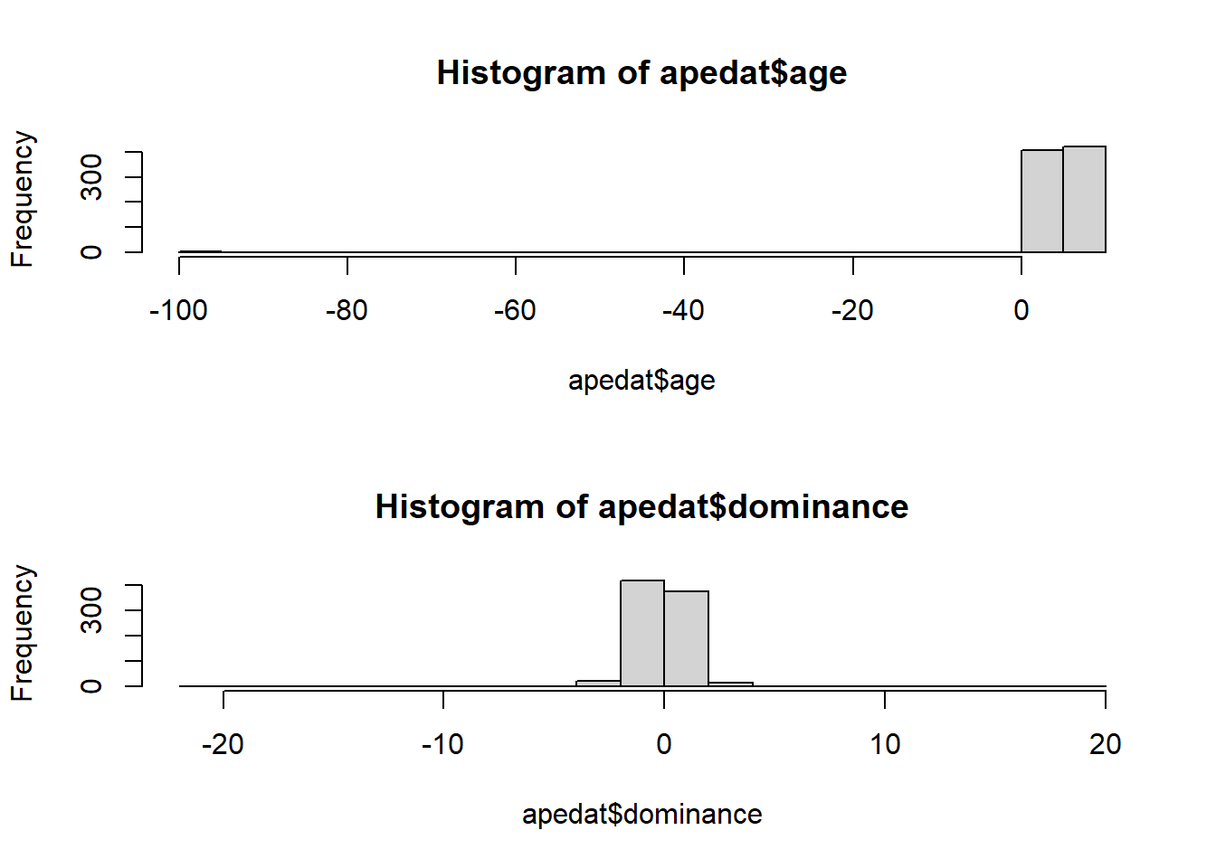
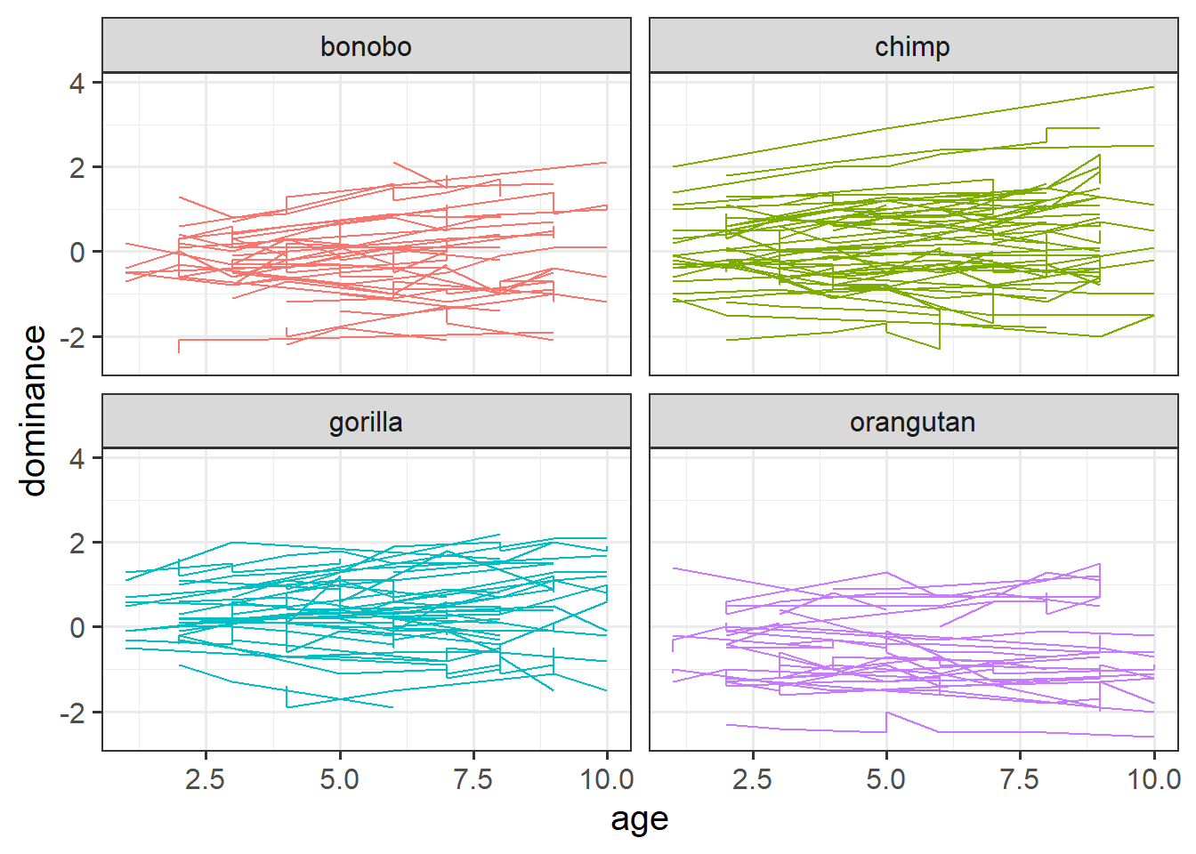
We have data from a large sample of great apes who have been studied between the ages of 1 to 10 years old (i.e. during adolescence). Our data includes 4 species of great apes: Chimpanzees, Bonobos, Gorillas and Orangutans. Each ape has been assessed on a primate dominance scale at various ages. Data collection was not very rigorous, so apes do not have consistent assessment schedules (i.e., one may have been assessed at ages 1, 3 and 6, whereas another at ages 2 and 8).

The researchers are interested in examining how the adolescent development of dominance in great apes differs between species.

Data on the dominance scores of the apes are available at https://uoepsy.github.io/data/lmm_apeage.csv and the information about which species each ape is are in https://uoepsy.github.io/data/lmm_apespecies.csv.

Table 1: Data Dictionary: lmm_apespecies.csv

variable	description
ape	Ape Name
species	Species (Bonobo, Chimpanzee, Gorilla, Orangutan)

Table 2: Data Dictionary: lmm_apeage.csv

variable	description
ape	Ape Name
age	Age at assessment (years)
dominance	Dominance (Z-scored)

Extra 12

Read in the data and check over it. Do any relevant cleaning/wrangling that might be necessary to put the datasets together into a single dataframe.

Solution 18. We’ll read in both datasets, and then join them together.

library(tidyverse)
library(lme4)
ape_species <- read_csv("https://uoepsy.github.io/data/lmm_apespecies.csv")
ape_age <- read_csv("https://uoepsy.github.io/data/lmm_apeage.csv")

Sometimes is handy to check that all our participants are in both datasets:

# are all the apes in ape_age also in ape_species?
all(ape_age$ape %in% ape_species$ape)

[1] TRUE

# and vice versa?
all(ape_species$ape %in% ape_age$ape)

[1] TRUE

Let’s join them:

apedat <- full_join(ape_age, ape_species)
head(apedat)

# A tibble: 6 × 4
  ape     age dominance species   
  <chr> <dbl>     <dbl> <chr>     
1 Joel      7       0.6 chimpanzee
2 Joel      5       1.2 chimpanzee
3 Joel      8       1.1 chimpanzee
4 Joel      1       0.2 chimpanzee
5 Joel      2       0.5 chimpanzee
6 Joel      6       1   chimpanzee

Solution 19. First off, we can see that we’ve got some weird typos. Some apes have been identified as “gorrila” but it is actually spelled “gorilla”.
Also, we’ve got people using two alternatives for the chimps: “chimp” and “chimpanzee”. We’ll need to combine those.

table(apedat$species)

    bonobo      chimp chimpanzee    gorilla    gorrila  orangutan 
       187        146        127        211          2        157 

Age looks like it has some weird values (possibly “-99”?), and there are possibly a few outliers in the dominance variable. Given that dominance is standardised, it is extremely unlikely that we would see values around 20. They’re not “impossible”, but they’re so incredibly unlikely that I’d be more comfortable assuming they are typos:

hist(apedat$age, breaks=20)
hist(apedat$dominance, breaks=20)

Just to see what the most extreme values of dominance are:

# show the biggest 5 absolute values in dominance variable
sort(abs(apedat$dominance), decreasing = TRUE)[1:5]

[1] 21.2 19.4  3.9  2.9  2.9

Solution 20.

apedat <- apedat |> 
  mutate(
    # fix species typos
    species = case_when(
      species %in% c("chimp","chimpanzee") ~ "chimp",
      species %in% c("gorilla","gorrila") ~ "gorilla",
      TRUE ~ species
    )
  ) |>
    filter(
      # get rid of ages -99
      age > 0, 
      # keep when dominance is between -5 and 5 
      # (5 here is a slightly arbitrary choice, but you can see from
      # our checks that this will only exclude the two extreme datapoints
      # that are 21.2 and 19.4
      (dominance < 5 & dominance > -5) 
    )

Extra 13

How is this data structure “hierarchical” (or “clustered”)? What are our level 1 units, and what are our level 2 units?

Solution 21. We have a random sample of \(\underbrace{\text{timepoints}}_{\text{level 1}}\) from a random sample of \(\underbrace{\text{apes}}_{\text{level 2}}\).

Extra 14

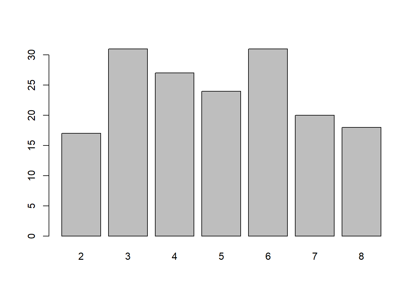
For how many apes do we have data? How many of each species?
How many datapoints does each ape have?

Hints

We’ve seen this last week too - counting the different levels in our data. There are lots of ways to do these things - functions like count(), summary(), n_distinct(), table(), mean(), min() etc. See 1: Group Structured Data #determining-sample-sizes

Solution 22. We have 168 apes in our dataset:

n_distinct(apedat$ape)

[1] 168

Here’s how many of each species:

apedat |> 
  group_by(species) |>
  summarise(
   n_apes = n_distinct(ape) 
  )

# A tibble: 4 × 2
  species   n_apes
  <chr>      <int>
1 bonobo        36
2 chimp         56
3 gorilla       46
4 orangutan     30

Let’s create a table of how many observations for each ape, and then we can create a table from that table, to show how many apes have 2 datapoints, how many have 3, 4, and so on:

table(apedat$ape) |>
  table() |>
  barplot()

Extra 15

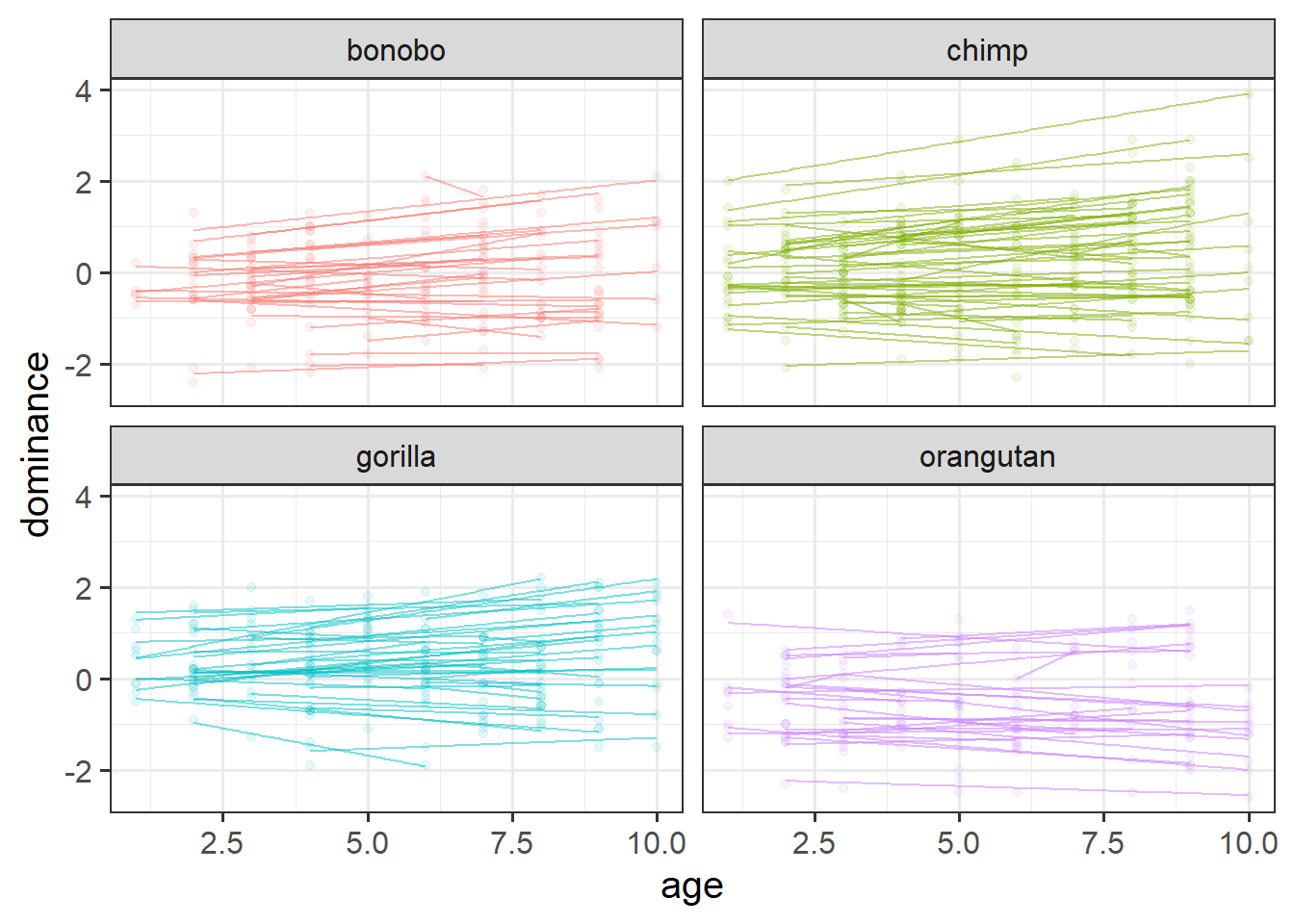
Make a plot to show how dominance changes as apes get older.

Hints

You might be tempted to use facet_wrap(~ape) here, but we have too many apes! The group aesthetic will probably help instead!

Solution 23. Here’s a line for each ape, and a facet for each species:

ggplot(apedat, aes(x = age, y = dominance, col = species))+
  geom_line(aes(group = ape)) + 
  facet_wrap(~species) + 
  guides(col="none")

It’s kind of hard to see the trend for each ape with the lines, so instead let’s plot points, and then make a separate little linear model for each ape:

ggplot(apedat, aes(x = age, y = dominance, col = species))+
  geom_point(alpha=.1) +
  stat_smooth(aes(group=ape),geom="line",method=lm,se=F,alpha=.5) +
  facet_wrap(~species) + 
  guides(col="none")

Extra 16

The youngest age that we have data for for any of our species is 1. But it’s often useful for the value 0 to be contained within the range of a predictor’s values, because that makes interpreting all the other estimates easier. (Why? Because the intercept, and all the group-level variability in intercepts, is estimated when the predictors = 0. And if 0 is outside of the range of predictors, then we’re estimating the intercept for values that don’t really exist in our data. Mathematically possible, but hard to interpret.)

For the current analysis, let’s subtract 1 from the age variable so that the minimum value of age becomes 0. In other words, let’s shift the age variable down by 1, so that the value 0 now represents the minimum age, 1. This way, the intercept (and the group-level variability in intercepts) will be estimated for the minimum age in our dataset.

Then fit a model that estimates the differences between primate species in how dominance changes over time.

Solution 24.

apedat$age <- apedat$age-1 

m.full <- lmer(dominance ~ 1 + age * species + (1 + age | ape), data = apedat)

Extra 17

Do primate species differ in the growth of dominance?
Perform an appropriate test/comparison.

Hints

This is asking about the age*species interaction, which in our model is represented by three parameters (the interaction terms between age and each of the three non-reference-level species). To assess the overall question, it might make more sense to do a model comparison.

Solution 25.

m.int <- lmer(dominance ~ 1 + age + species + (1 + age | ape), data = apedat)
m.full <- lmer(dominance ~ 1 + age * species + (1 + age | ape), data = apedat)

anova(m.int, m.full)

Data: apedat
Models:
m.int: dominance ~ 1 + age + species + (1 + age | ape)
m.full: dominance ~ 1 + age * species + (1 + age | ape)
       npar AIC BIC logLik -2*log(L) Chisq Df Pr(>Chisq)   
m.int     9 807 849   -394       789                       
m.full   12 801 858   -389       777  11.5  3     0.0092 **
---
Signif. codes:  0 '***' 0.001 '**' 0.01 '*' 0.05 '.' 0.1 ' ' 1

Species differ in how dominance changes over adolescence (\(\chi^2(3) = 11.52, p = 0.009\)).

Extra 18

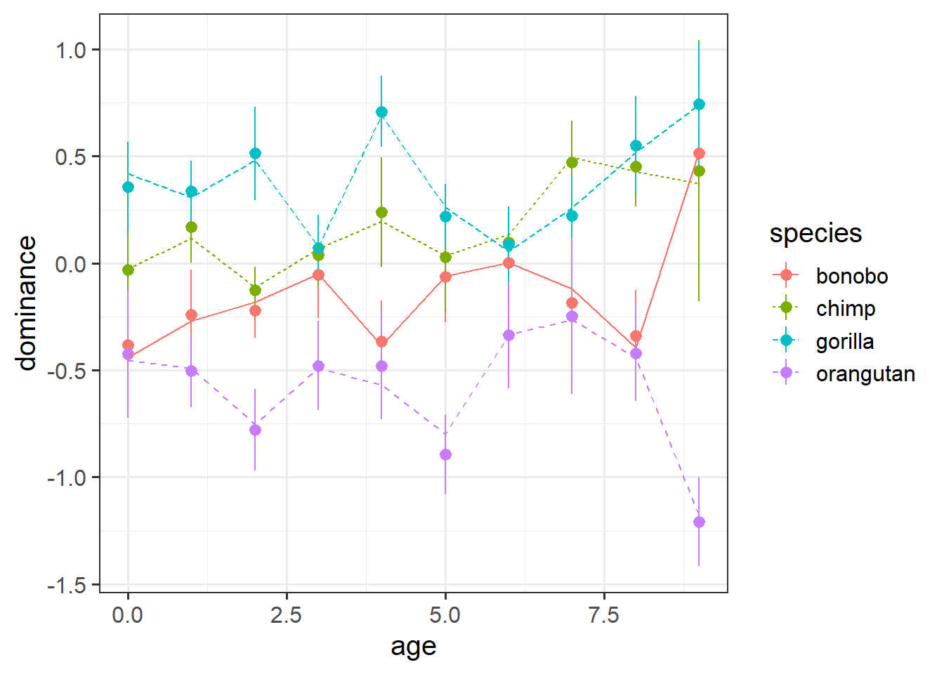
Below is code that creates a plot of the average model predicted values for each age.¹

Before you run the code - do you expect to see straight lines? (remember, not every ape is measured at age 2, or age 3, etc).

library(broom.mixed)

augment(m.full) |>
  ggplot(aes(age,dominance, color=species)) +
  # the point ranges are our observations
  stat_summary(fun.data=mean_se, geom="pointrange") + 
  # the lines are the average of our predictions  
  stat_summary(aes(y=.fitted, linetype=species), fun=mean, geom="line")

Solution 26. Averaging fitted values would give us straight lines if every ape had data at all ages, but in our study we have some apes with only 2 data points, and each ape has different set of ages (e.g., one ape might be measured at age 3, 6, and 10, another ape might be at ages 2 and 16).

So the average prediction of orangutans at age 10 might be based on only 3 orangutans, whereas the average prediction of orangutans might be based on 20 orangutans.

library(broom.mixed)
augment(m.full) |>
ggplot(aes(age,dominance, color=species)) +
  # the point ranges are our observations
  stat_summary(fun.data=mean_se, geom="pointrange") + 
  # the lines are the average of our predictions  
  stat_summary(aes(y=.fitted, linetype=species), fun=mean, geom="line")

Extra 19

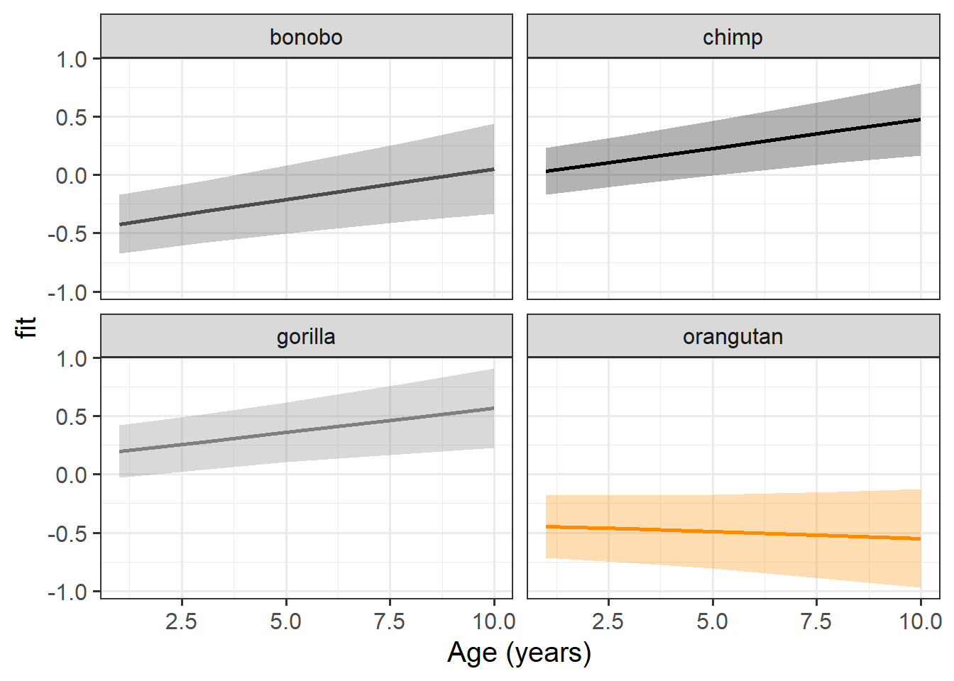
Plot the model based fixed effects.

Hints

This should get you started:

library(effects)
effect(term = "age*species", mod = m.full) |>
  as.data.frame() |>
  ggplot( 
    ...
    ...

Solution 27. Here’s my attempt:

library(effects)
effect(term = "age*species", mod = m.full) |>
  as.data.frame() |>
  ggplot(aes(x=age+1,y=fit,col=species))+
  geom_line(lwd=1)+
  geom_ribbon(aes(ymin=lower,ymax=upper,fill=species),col=NA,alpha=.3) +  
  scale_color_manual(values=c("grey30","black","grey50","darkorange")) +
  scale_fill_manual(values=c("grey30","black","grey50","darkorange")) +
  facet_wrap(~species) + 
  guides(col="none",fill="none") +
  labs(x="Age (years)")

Extra 20

Interpret each of the fixed effects from the model (you might also want to get some p-values or confidence intervals).

Hints

Each of the estimates should correspond to part of our plot from the previous question.

You can either use the lmerTest::lmer() to get p-values, or why not try using confint(model) to get some confidence intervals.

Solution 28. Let’s get some confidence intervals:

Remember - a confidence interval is a range of plausible values for the thing we are estimating. The statistical significance we are used to with p-values of \(p < .05\) is when the 95% confidence interval does not contain zero (and \(p > .05\) is when the interval does contain zero).²

Here the parm = "beta_" bit just tells the function that we want intervals only for our fixed effects:

confint(m.full, parm = "beta_")

                       2.5 %  97.5 %
(Intercept)          -0.6707 -0.1730
age                   0.0236  0.0814
specieschimp          0.1338  0.7701
speciesgorilla        0.2812  0.9493
speciesorangutan     -0.3891  0.3426
age:specieschimp     -0.0397  0.0339
age:speciesgorilla   -0.0501  0.0280
age:speciesorangutan -0.1063 -0.0217

term	est	CI	interpretation
(Intercept)	-0.42	[-0.67, -0.17]*	estimated dominance of 1 year old bonobos (at left hand side of plot, bonobo line is lower than 0)
age	0.05	[0.02, 0.08]*	estimated change in dominance score for every year older a bonobo gets (slope of bonobo line)
specieschimp	0.45	[0.13, 0.77]*	estimated difference in dominance scores at age 1 between bonobos and chimps (at left hand side of plot, chimp line is higher than bonobo line)
speciesgorilla	0.62	[0.28, 0.95]*	estimated difference in dominance scores at age 1 between bonobos and gorillas (at left hand side of plot, gorilla line is higher than bonobo line)
speciesorangutan	-0.02	[-0.39, 0.34]	no significant difference in dominance scores at age 1 between bonobos and orangutans (at the left hand side of our plot, orangutan line is similar height to bonobo line)
age:specieschimp	0.00	[-0.04, 0.03]	no significant difference between chimps and bonobos in the change in dominance for every year older (slope of chimp line is similar to slope of bonobo line)
age:speciesgorilla	-0.01	[-0.05, 0.03]	no significant difference between gorillas and bonobos in the change in dominance for every year older (slope of gorilla line is similar to slope of bonobo line)
age:speciesorangutan	-0.06	[-0.11, -0.02]*	estimated difference between orangutans and bonobos in the change in dominance for every year older (slope of orangutan line is less steep than slope of bonobo line)

Footnotes

1. This is like taking predict() from the model, and then then grouping by age, and calculating the mean of those predictions. However, we can do this more easily using augment() and then some fancy stat_summary() in ggplot

2. provided that the confidence intervals and p-values are constructed using the same methods