Simple Linear Regression

Learning Objectives

At the end of this lab, you will:

1. Be able to specify a simple linear model.
2. Understand what fitted values and residuals are.
3. Be able to interpret the coefficients of a fitted model.

Requirements

1. Be up to date with lectures from Weeks 1 & 2
2. Have completed Week 1 lab exercises

Required R Packages

Remember to load all packages within a code chunk at the start of your RMarkdown file using library(). If you do not have a package and need to install, do so within the console using install.packages(" "). For further guidance on installing/updating packages, see Section C here.

For this lab, you will need to load the following package(s):

• tidyverse
• sjPlot

Lab Data

You can download the data required for this lab here or read it in via this link https://uoepsy.github.io/data/riverview.csv.

Study Overview

Research Question

Is there an association between income and education level in the city of Riverview?

Let’s imagine a study into income disparity for workers in a local authority. We might carry out interviews and find that there is an association between the level of education and an employee’s income. Those with more formal education seem to be better paid.

In this lab, we will use the riverview data (see below codebook) to examine whether education level is related to income among the employees working for the city of Riverview, a hypothetical midwestern city in the US.

Riverview data codebook.

Description

The riverview data come from Lewis-Beck and Lewis-Beck (2015) and contain five attributes collected from a random sample of employees working in the hypothetical city of Riverview (\(n=32\)). The attributes include:

• education: Years of formal education
• income: Annual income (in thousands of U.S. dollars)
• seniority: Years of seniority
• gender: Employee’s gender
• male: Dummy coded gender variable (0 = Female, 1 = Male)
• party: Political party affiliation

Preview

The first six rows of the data are:

education	income	seniority	gender	male	party
8	37.449	7	male	1	Democrat
8	26.430	9	female	0	Independent
10	47.034	14	male	1	Democrat
10	34.182	16	female	0	Independent
10	25.479	1	female	0	Republican
12	46.488	11	female	0	Democrat

Setup

Setup

1. Create a new RMarkdown file
2. Load the required package(s)
3. Read the riverview dataset into R, assigning it to an object named riverview

Solution

#Loading the required package(s)
library(tidyverse)
library(sjPlot)

#Reading in riverview data and storing in object named 'riverview'
riverview <- read_csv("https://uoepsy.github.io/data/riverview.csv")

#check first six rows
head(riverview)

# A tibble: 6 × 6
  education income seniority gender  male party      
      <dbl>  <dbl>     <dbl> <chr>  <dbl> <chr>      
1         8   37.4         7 male       1 Democrat   
2         8   26.4         9 female     0 Independent
3        10   47.0        14 male       1 Democrat   
4        10   34.2        16 female     0 Independent
5        10   25.5         1 female     0 Republican 
6        12   46.5        11 female     0 Democrat   

Exercises

Data Exploration

The common first port of call for almost any statistical analysis is to explore the data, and we can do this visually and/or numerically.

================ Description	Marginal Distributions The distribution of each variable (e.g., employee incomes and education levels) without reference to the values of the other variables	Bivariate Associations Describing the relationship between two numeric variables
Visually	Plot each variable individually. You could use, for example, geom_density() for a density plot or geom_histogram() for a histogram to comment on and/or examine: The shape of the distribution. Look at the shape, centre and spread of the distribution. Is it symmetric or skewed? Is it unimodal or bimodal? Identify any unusual observations. Do you notice any extreme observations (i.e., outliers)?	Plot associations among two variables. | | | You could use, for example, geom_point() for a scatterplot to comment on and/or examine: | | The direction of the association indicates whether there is a positive or negative association The form of association refers to whether the relationship between the variables can be summarized well with a straight line or some more complicated pattern The strength of association entails how closely the points fall to a recognizable pattern such as a line Unusual observations that do not fit the pattern of the rest of the observations and which are worth examining in more detail
Numerically	Compute and report summary statistics e.g., mean, standard deviation, median, min, max, etc. You could, for example, calculate summary statistics such as the mean (mean()) and standard deviation (sd()), etc. within summarize()	Compute and report the correlation coefficient. You can use the cor() function to calculate this

Marginal Distributions

Question 2

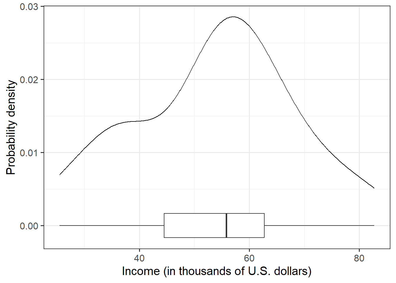
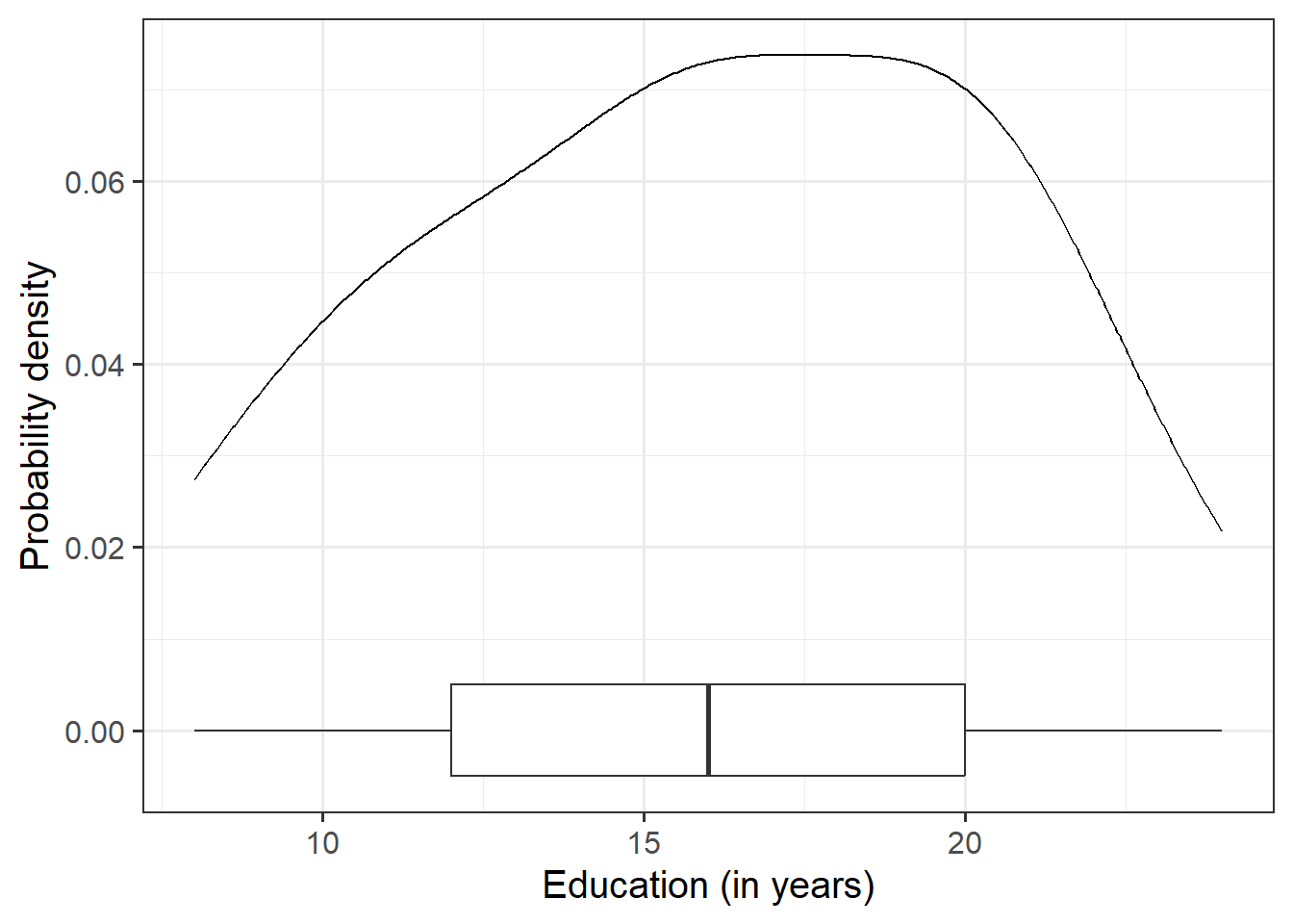
Visualise and describe the marginal distributions of employee incomes and education level.

Solution

Employee Incomes

Visualisation of distribution:

ggplot(data = riverview, aes(x = income)) +
  geom_density() +
  geom_boxplot(width = 1/300) +
  labs(x = "Income (in thousands of U.S. dollars)", 
       y = "Probability density")

Figure 1: Density plot and boxplot of employee incomes

Initial observations from plot:

• The distribution of employee incomes was unimodal
• Most of the incomes were between roughly $45,000 and $63,000
• The lowest income in the sample was approximately $25,000 and the highest approximately $83,000. This suggested there was a fair high degree of variation in the data.
• The boxplot did not highlight any outliers in the data.

Descriptive (or summary) statistics for the employees’ incomes:

desc_income <- riverview %>% 
  summarize(
    M = mean(income), 
    SD = sd(income)
    )
desc_income

# A tibble: 1 × 2
      M    SD
  <dbl> <dbl>
1  53.7  14.6

Following the exploration above, we can describe the income variable as follows:

The marginal distribution of income was unimodal with a mean of approximately $53,700. There was variation in employees’ salaries (SD = $14,553).

Employee Education Levels

Visualisation of distribution:

ggplot(data = riverview, aes(x = education)) +
  geom_density() +
  geom_boxplot(width = 1/100) +
  labs(x = "Education (in years)", 
       y = "Probability density")

Figure 2: Density plot and boxplot of employee education levels

Initial observations from plot:

• The distribution of employee education was unimodal
• Most of the employees received formal education for between 12 and 20 years
• The fewest formal years of education was approximately 8 years, and the highest approximately 25. This suggested there was a fair high degree of variation in the data.
• The boxplot did not highlight any outliers in the data

Descriptive (or summary) statistics for the employees’ level of education:

desc_education <- riverview %>%
  summarize(
    M = mean(education),
    SD = sd(education)
    )
desc_education

# A tibble: 1 × 2
      M    SD
  <dbl> <dbl>
1    16  4.36

Following the exploration above, we can describe the education variable as follows:

The marginal distribution of education was unimodal with an average of of 16 years. There was variation in employees’ level of education (SD = 4.4 years).

Associations among Variables

Question 3

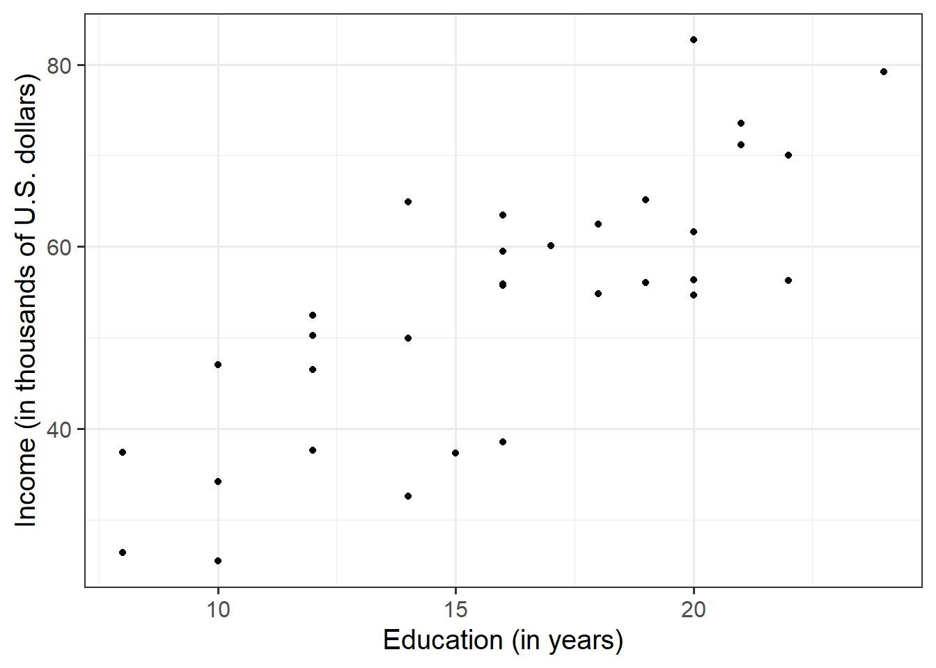
Create a scatterplot of income and education level before calculating the correlation between income and education level.

Making reference to both the plot and correlation coefficient, describe the association between income and level of education among the employees in the sample.

Hint

We are trying to investigate how income varies when varying years of formal education. Hence, income is the dependent variable (on the y-axis), and education is the independent variable (on the x-axis).

Solution

Let’s produce a scatterplot:

ggplot(data = riverview, aes(x = education, y = income)) +
  geom_point() +
  labs(x = "Education (in years)", 
       y = "Income (in thousands of U.S. dollars)")

Figure 3: The association between employees’ education level and income

To comment on the strength of the linear association we compute the correlation coefficient:

corr <- riverview %>%
  select(education, income) %>%
  cor()
corr

          education    income
education 1.0000000 0.7947847
income    0.7947847 1.0000000

that is, \[ r_{\text({education, income})} = 0.79 \]

There was a strong positive linear association between education level and income for the employees in the sample. High incomes tended to be observed, on average, with more years of formal education (\(r\) = .79).

Model Specification and Fitting

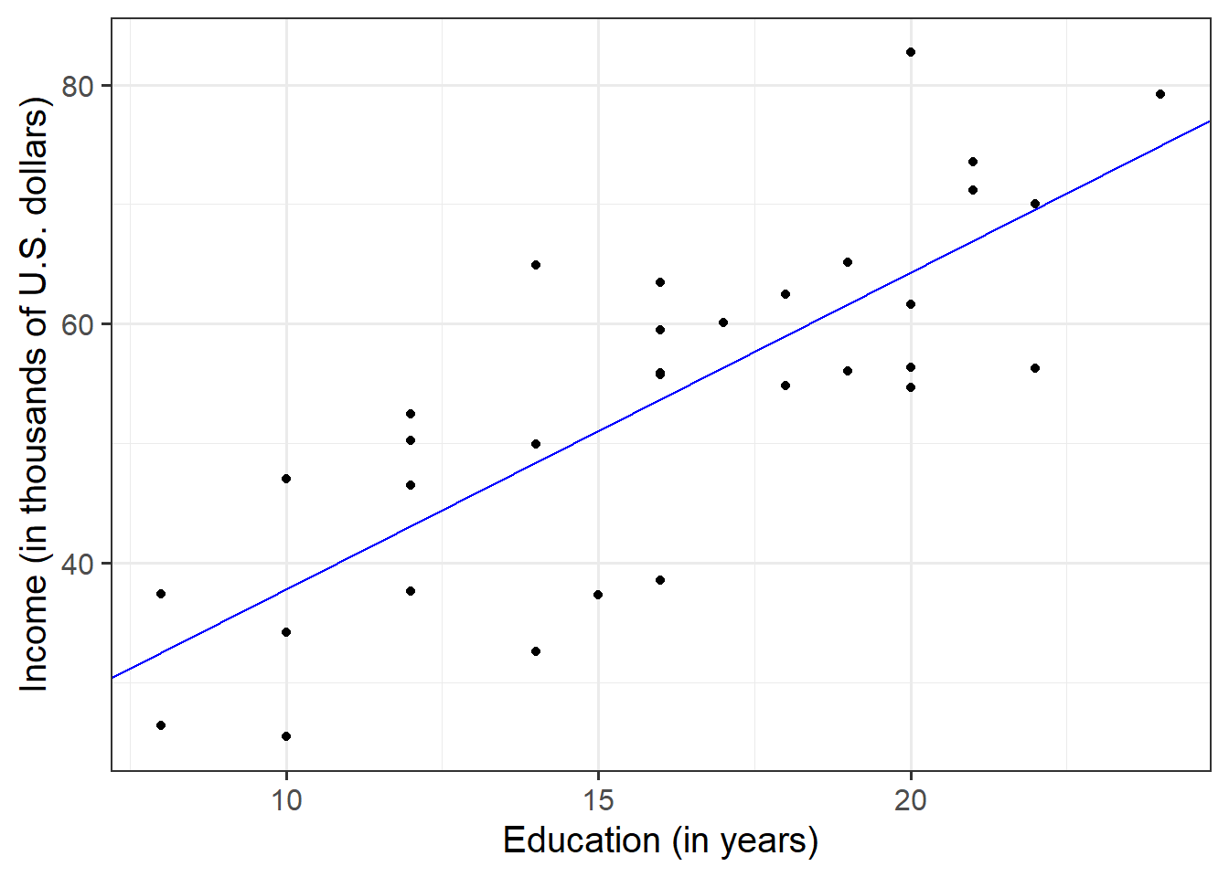
The scatterplot highlighted a linear relationship, where the data points were scattered around an underlying linear pattern with a roughly-constant spread as x varied.

Hence, we will try to fit a simple (i.e., one x variable only) linear regression model:

\[ y_i = \beta_0 + \beta_1 x_i + \epsilon_i \\ \quad \text{where} \quad \epsilon_i \sim N(0, \sigma) \text{ independently} \]

What does \(y_i = \beta_0 + \beta_1 x_i + \epsilon_i \quad \text{where} \quad \epsilon_i \sim N(0, \sigma) \text{ independently}\) mean?

Lets break the statement down into smaller parts:

\(y_i = \beta_0 + \beta_1 x_i + \epsilon_i\)

• \(y_i\) is our measured outcome variable (our DV)
• \(x_i\) is our measured predictor variable (our IV)
• \(\beta_0\) is the model intercept
• \(\beta_1\) is the model slope

\(\epsilon \sim N(0, \sigma) \text{ independently}\)

• \(\epsilon\) is the residual error
• \(\sim\) means ‘distributed according to’
• \(\sim N(0, \sigma) \text{ independently}\) means ‘normal distribution with a mean of 0 and a variance of \(\sigma\)’
• Together, we can say that the errors around the line have a mean of zero and constant spread as x varies.

Question 4

First, write the equation of the fitted line.

Next, using the lm() function, fit a simple linear model to predict income (DV) by Education (IV), naming the output mdl.

Lastly, add update your equation of the fitted line to include the estimated coefficients.

Hint

The syntax of the lm() function is:

[model name] <- lm([response variable i.e., dependent variable] ~ [explanatory variable i.e., independent variable], data = [dataframe])

Solution

First, lets specify the fitted model, which can be written either as:

Option A

\[ \widehat{Income} = \hat \beta_0 + \hat \beta_1 \cdot Education \]

Option B

\[ \widehat{Income} = \hat \beta_0 \cdot 1 + \hat \beta_1 \cdot Education \]

To fit the model in R, as the variables are in the riverview dataframe, we would write:

Option A

mdl <- lm(income ~ education, data = riverview)
mdl

Call:
lm(formula = income ~ education, data = riverview)

Coefficients:
(Intercept)    education  
     11.321        2.651  

Option B

mdl <- lm(income ~ 1 + education, data = riverview)
mdl

Call:
lm(formula = income ~ 1 + education, data = riverview)

Coefficients:
(Intercept)    education  
     11.321        2.651  

Why is there a 1 in the Option B’s?

When we specify the linear model in R, we include after the tilde sign (\(\sim\)), the variables that appear to the right of the \(\hat \beta\)s. The intercept, or \(\beta_0\), is a constant. That is, we could write it as multiplied by 1.

Including the 1 explicitly is not necessary because it is included by default (you can check this by comparing the outputs of A & B above with and without the 1 included - the estimates are the same!). After a while, you will find you just want to drop the 1 (i.e., Option B) when calling lm() because you know that it’s going to be there, but in these early weeks we tried to keep it explicit to make it clear that you want to the intercept to be estimated.

Note that by calling the name of the fitted model, mdl, you can see the estimated regression coefficients \(\hat \beta_0\) and \(\hat \beta_1\). We can add these values to the fitted line:

\[ \widehat{Income} = 11.32 + 2.65 \cdot Education \\ \]

Question 5

Explore the following equivalent ways to obtain the estimated regression coefficients — that is, \(\hat \beta_0\) and \(\hat \beta_1\) — from the fitted model:

• mdl
• mdl$coefficients
• coef(mdl)
• coefficients(mdl)
• summary(mdl)

Solution

The estimated parameters returned by the below methods are all equivalent. However, summary() returns more information.

mdl()

Simply invoke the name of the fitted model:

mdl

Call:
lm(formula = income ~ 1 + education, data = riverview)

Coefficients:
(Intercept)    education  
     11.321        2.651  

mdl$coefficients

mdl$coefficients

(Intercept)   education 
  11.321379    2.651297 

coef(mdl)

coef(mdl)

(Intercept)   education 
  11.321379    2.651297 

coefficients(mdl)

coefficients(mdl)

(Intercept)   education 
  11.321379    2.651297 

summary(mdl)

Look under the “Estimate” column:

summary(mdl)

Call:
lm(formula = income ~ 1 + education, data = riverview)

Residuals:
    Min      1Q  Median      3Q     Max 
-15.809  -5.783   2.088   5.127  18.379 

Coefficients:
            Estimate Std. Error t value Pr(>|t|)    
(Intercept)  11.3214     6.1232   1.849   0.0743 .  
education     2.6513     0.3696   7.173 5.56e-08 ***
---
Signif. codes:  0 '***' 0.001 '**' 0.01 '*' 0.05 '.' 0.1 ' ' 1

Residual standard error: 8.978 on 30 degrees of freedom
Multiple R-squared:  0.6317,    Adjusted R-squared:  0.6194 
F-statistic: 51.45 on 1 and 30 DF,  p-value: 5.562e-08

The estimated intercept is \(\hat \beta_0 = 11.32\) and the estimated slope is \(\hat \beta_1 = 2.65\).

Question 6

Explore the following equivalent ways to obtain the estimated standard deviation of the errors — that is, \(\hat \sigma\) — from the fitted model mdl:

• sigma(mdl)
• summary(mdl)

Huh? What is \(\sigma\)?

The standard deviation of the errors, denoted by \(\sigma\), is an important quantity that our model estimates. It represents how much individual data points tend to deviate above and below the regression line.

A small \(\sigma\) indicates that the points hug the line closely and we should expect fairly accurate predictions, while a large \(\sigma\) suggests that, even if we estimate the line perfectly, we can expect individual values to deviate from it by substantial amounts.

The estimated standard deviation of the errors is denoted \(\hat \sigma\), and is estimated by essentially averaging squared residuals (giving the variance) and taking the square-root:

\[ \begin{align} & \hat \sigma = \sqrt{\frac{SS_{Residual}}{n - k - 1}} \\ \qquad \\ & \text{where} \\ & SS_{Residual} = \textrm{Sum of Squared Residuals} = \sum_{i=1}^n{(\epsilon_i)^2} \end{align} \]

Solution

The estimated standard deviation of the errors can be equivalently obtained by the below methods. However, summary() returns more information.

sigma(mdl)

sigma(mdl)

[1] 8.978116

summary(mdl)

Look at the “Residual standard error” entry of the summary(mdl) output:

summary(mdl)

Call:
lm(formula = income ~ 1 + education, data = riverview)

Residuals:
    Min      1Q  Median      3Q     Max 
-15.809  -5.783   2.088   5.127  18.379 

Coefficients:
            Estimate Std. Error t value Pr(>|t|)    
(Intercept)  11.3214     6.1232   1.849   0.0743 .  
education     2.6513     0.3696   7.173 5.56e-08 ***
---
Signif. codes:  0 '***' 0.001 '**' 0.01 '*' 0.05 '.' 0.1 ' ' 1

Residual standard error: 8.978 on 30 degrees of freedom
Multiple R-squared:  0.6317,    Adjusted R-squared:  0.6194 
F-statistic: 51.45 on 1 and 30 DF,  p-value: 5.562e-08

Note

The term “Residual standard error” is a misnomer, as the help page for sigma says (check ?sigma). However, it’s hard to get rid of this bad name as it has been used in too many books showing R output.

The estimated standard deviation of the errors is \(\hat \sigma = 8.98\).

Question 7

Interpret the estimated intercept, slope, and standard deviation of the errors in the context of the research question.

Hint

To interpret the estimated standard deviation of the errors we can use the fact that about 95% of values from a normal distribution fall within two standard deviations of the centre.

Solution

Intercept

The estimated income associated to zero years of formal education is $11,321.

Slope

The estimated increase in income associated to a one year increase in education is $2,651.

Standard deviation of the errors

For any particular level of education, employee incomes should be distributed above and below the regression line with standard deviation estimated to be \(\hat \sigma = 8.98\). Since \(2 \hat \sigma = 2 (8.98) = 17.96\), we expect most (about 95%) of the employee incomes to be within about $18,000 from the regression line.

Question 8

Plot the data and the fitted regression line. To do so:

• Extract the estimated regression coefficients e.g., via betas <- coef(mdl)
• Extract the first entry of betas (i.e., the intercept) via betas[1]
• Extract the second entry of betas (i.e., the slope) via betas[2]
• Provide the intercept and slope to the function

Hint

Extracting values: The function coef(mdl) returns a vector: that is, a sequence of numbers all of the same type. To get the first element of the sequence you append [1], and [2] for the second.

Plotting: In your ggplot(), you will need to specify geom_abline(). This might help get you started:

geom_abline(intercept = <intercept>, slope = <slope>)

Solution

First extract the values required:

betas <- coef(mdl)
intercept <- betas[1]
slope <- betas[2]

We can plot the model as follows:

ggplot(data = riverview, aes(x = education, y = income)) +
  geom_point() +
  geom_abline(intercept = intercept, slope = slope, color = 'blue') + 
  labs(x = "Education (in years)", y = "Income (in thousands of U.S. dollars)")

Predicted Values & Residuals

Predicted Values

Model predicted values for sample data:

We can get out the model predicted values for \(y\), the “y hats” (\(\hat y\)), for the data in the sample using various functions:

• predict(<fitted model>)
• fitted(<fitted model>)
• fitted.values(<fitted model>)
• mdl$fitted.values

For example, this will give us the estimated income (point on our regression line) for each observed value of education level.

predict(mdl)

       1        2        3        4        5        6        7        8 
32.53175 32.53175 37.83435 37.83435 37.83435 43.13694 43.13694 43.13694 
       9       10       11       12       13       14       15       16 
43.13694 48.43953 48.43953 48.43953 51.09083 53.74212 53.74212 53.74212 
      17       18       19       20       21       22       23       24 
53.74212 53.74212 56.39342 59.04472 59.04472 61.69601 61.69601 64.34731 
      25       26       27       28       29       30       31       32 
64.34731 64.34731 64.34731 66.99861 66.99861 69.64990 69.64990 74.95250 

Model predicted values for other (unobserved) data:

To compute the model-predicted values for unobserved data (i.e., data not contained in the sample), we can use the following function:

• predict(<fitted model>, newdata = <dataframe>)

For this example, we first need to remember that the model predicts income using the independent variable education. Hence, if we want predictions for new (unobserved) data, we first need to create a tibble with a column called education containing the years of education for which we want the prediction, and store this as a dataframe.

#Create dataframe 'newdata' containing education years of 7, 11 and 25
newdata <- tibble(education = c(7, 11, 25))
newdata

# A tibble: 3 × 1
  education
      <dbl>
1         7
2        11
3        25

Then we take newdata and add a new column called income_hat, computed as the prediction from the fitted mdl using the newdata above:

newdata <- newdata %>%
  mutate(
    income_hat = predict(mdl, newdata = newdata)
  )
newdata

# A tibble: 3 × 2
  education income_hat
      <dbl>      <dbl>
1         7       29.9
2        11       40.5
3        25       77.6

Residuals

The residuals represent the deviations between the actual responses and the predicted responses and can be obtained either as

• mdl$residuals
• resid(mdl)
• residuals(mdl)
• computing them as the difference between the response (\(y_i\)) and the predicted response (\(\hat y_i\))

Question 9

Use predict(mdl) to compute the fitted values and residuals. Mutate the riverview dataframe to include the fitted values and residuals as extra columns.

Assign to the following symbols the corresponding numerical values:

• \(y_{3}\) (response variable for unit \(i = 3\) in the sample data)
• \(\hat y_{3}\) (fitted value for the third unit)
• \(\hat \epsilon_{5}\) (the residual corresponding to the 5th unit, i.e., \(y_{5} - \hat y_{5}\))

Solution

riverview_fitted <- riverview %>%
  mutate(
    income_hat = predict(mdl),
    resid = income - income_hat
  )

head(riverview_fitted)

# A tibble: 6 × 8
  education income seniority gender  male party       income_hat  resid
      <dbl>  <dbl>     <dbl> <chr>  <dbl> <chr>            <dbl>  <dbl>
1         8   37.4         7 male       1 Democrat          32.5   4.92
2         8   26.4         9 female     0 Independent       32.5  -6.10
3        10   47.0        14 male       1 Democrat          37.8   9.20
4        10   34.2        16 female     0 Independent       37.8  -3.65
5        10   25.5         1 female     0 Republican        37.8 -12.4 
6        12   46.5        11 female     0 Democrat          43.1   3.35

• \(y_{3}\) = 47.03 (see row 3, column 2)
• \(\hat y_{3}\) = 37.83 (see row 3, column 7)
• \(\hat \epsilon_{5} = y_{5} - \hat y_{5}\) = -12.36 (see row 5, columns 2 and 7)

Question 10

Describe the design of the study, and the analyses that you undertook. Interpret your results in the context of the research question and report your model results in full.

Provide key model results in a formatted table.

Hint

Use tab_model() from the sjPlot package.

Remember that you can rename your DV and IV labels by specifying dv.labels and pred.labels.

Make sure to write your results up following APA guidelines

Solution

Before we write up our analyses & results, lets first create the table of results:

tab_model(mdl,
          dv.labels = "Income (in thousands of US dollars)",
          pred.labels = c("education" = "Education (years)"),
          title = "Regression Table for Income Model")

Table 1: Regression Table for Income Model

	Income (in thousands of US dollars)
Predictors	Estimates	CI	p
(Intercept)	11.32	-1.18 – 23.83	0.074
Education (years)	2.65	1.90 – 3.41	<0.001
Observations	32
R2 / R2 adjusted	0.632 / 0.619

The riverview dataset contained information on 32 participants who worked in the hypothetical city of Riverview, US. Using a between-subjects design, the researchers collected information on participants’ sex, income, education, and seniority level.

To investigate whether there was an association between income and education level, the following simple linear regression model was used:

\[ \text{Income}= \beta_0 + \beta_1 \cdot \text{Education} \]

Full regression results are displayed in Table 1. The estimated income associated with no formal years of education was $11,321. Each additional year of formal education was associated with an income increase of $2,651.

References

Lewis-Beck, Colin, and Michael Lewis-Beck. 2015. Applied Regression: An Introduction. Vol. 22. Sage publications.