Multiple Linear Regression

Learning Objectives

At the end of this lab, you will:

1. Extend the ideas of single linear regression to consider regression models with two or more predictors
2. Understand and interpret the coefficients in multiple linear regression models

Requirements

1. Be up to date with lectures
2. Have completed Week 1 and Week 2 lab exercises

Required R Packages

Remember to load all packages within a code chunk at the start of your RMarkdown file using library(). If you do not have a package and need to install, do so within the console using install.packages(" "). For further guidance on installing/updating packages, see Section C here.

For this lab, you will need to load the following package(s):

• tidyverse
• patchwork
• sjPlot
• kableExtra

Lab Data

You can download the data required for this lab here or read it in via this link https://uoepsy.github.io/data/wellbeing.csv.

Study Overview

Research Question

Is there an association between wellbeing and time spent outdoors after taking into account the association between wellbeing and social interactions?

Wellbeing/Rurality data codebook.

Description

From the Edinburgh & Lothians, 100 city/suburb residences and 100 rural residences were chosen at random and contacted to participate in the study. The Warwick-Edinburgh Mental Wellbeing Scale (WEMWBS), was used to measure mental health and wellbeing.

Participants filled out a questionnaire including items concerning: estimated average number of hours spent outdoors each week, estimated average number of social interactions each week (whether on-line or in-person), whether a daily routine is followed (yes/no). For those respondents who had an activity tracker app or smart watch, they were asked to provide their average weekly number of steps.

The data in wellbeing.csv contain seven attributes collected from a random sample of \(n=200\) hypothetical residents over Edinburgh & Lothians, and include:

• wellbeing: Warwick-Edinburgh Mental Wellbeing Scale (WEMWBS), a self-report measure of mental health and well-being. The scale is scored by summing responses to each item, with items answered on a 1 to 5 Likert scale. The minimum scale score is 14 and the maximum is 70.
  
• outdoor_time: Self report estimated number of hours per week spent outdoors
  
• social_int: Self report estimated number of social interactions per week (both online and in-person)
• routine: Binary 1=Yes/0=No response to the question “Do you follow a daily routine throughout the week?”
• location: Location of primary residence (City, Suburb, Rural)
• steps_k: Average weekly number of steps in thousands (as given by activity tracker if available)
• age: Age in years of respondent

Preview

The first six rows of the data are:

age	outdoor_time	social_int	routine	wellbeing	location	steps_k
28	12	13	1	36	rural	21.6
56	5	15	1	41	rural	12.3
25	19	11	1	35	rural	49.8
60	25	15	0	35	rural	NA
19	9	18	1	32	rural	48.1
34	18	13	1	34	rural	67.3

Setup

Setup

1. Create a new RMarkdown file
2. Load the required package(s)
3. Read the wellbeing dataset into R, assigning it to an object named mwdata

Solution

#Loading the required package(s)
library(tidyverse)
library(patchwork)
library(sjPlot)
library(kableExtra)

# Reading in data and storing to an object named 'mwdata'
mwdata <- read_csv("https://uoepsy.github.io/data/wellbeing_rural.csv")

Exercises

Study & Analysis Plan Overview

Question 1

Provide a brief overview of the study design and data, before detailing your analysis plan to address the research question.

Hint

• Give the reader some background on the context of the study (you might be able to re-use some of the content you wrote for Lab 1 here)
• State what type of analysis you will conduct in order to address the research question
• Specify the model to be fitted to address the research question
• Specify your chosen significance (\(\alpha\)) level
• State your hypotheses

Solution

The mwdata dataset contained information on 200 hypothetical participants who lived in Edinburgh & Lothians area. Using a between-subjects design, the researchers collected information on participants’ wellbeing (measured via WEMWBS), outdoor time (hours per week), social interactions (number per week), routine (whether or not one was followed), location of residence (City, Suburb, or Rural), average weekly steps (in thousands), and age (in years).

To address the research question of whether there is an association between wellbeing and time spent outdoors after taking into account the association between wellbeing and social interactions, we are going to fit the following multiple linear regression model:

\[ \text{Wellbeing} = \beta_0 + \beta_1 \cdot Social Interactions + \beta_2 \cdot Outdoor Time \]

Effects will be considered statistically significant at \(\alpha=.05\).

Our hypotheses are:

\(H_0: \beta_2 = 0\): There is no association between well-being and time spent outdoors after taking into account the association between well-being and social interactions

\(H_1: \beta_2 \neq 0\): There is an association between well-being and time spent outdoors after taking into account the association between well-being and social interactions

Descriptive Statistics

Question 2

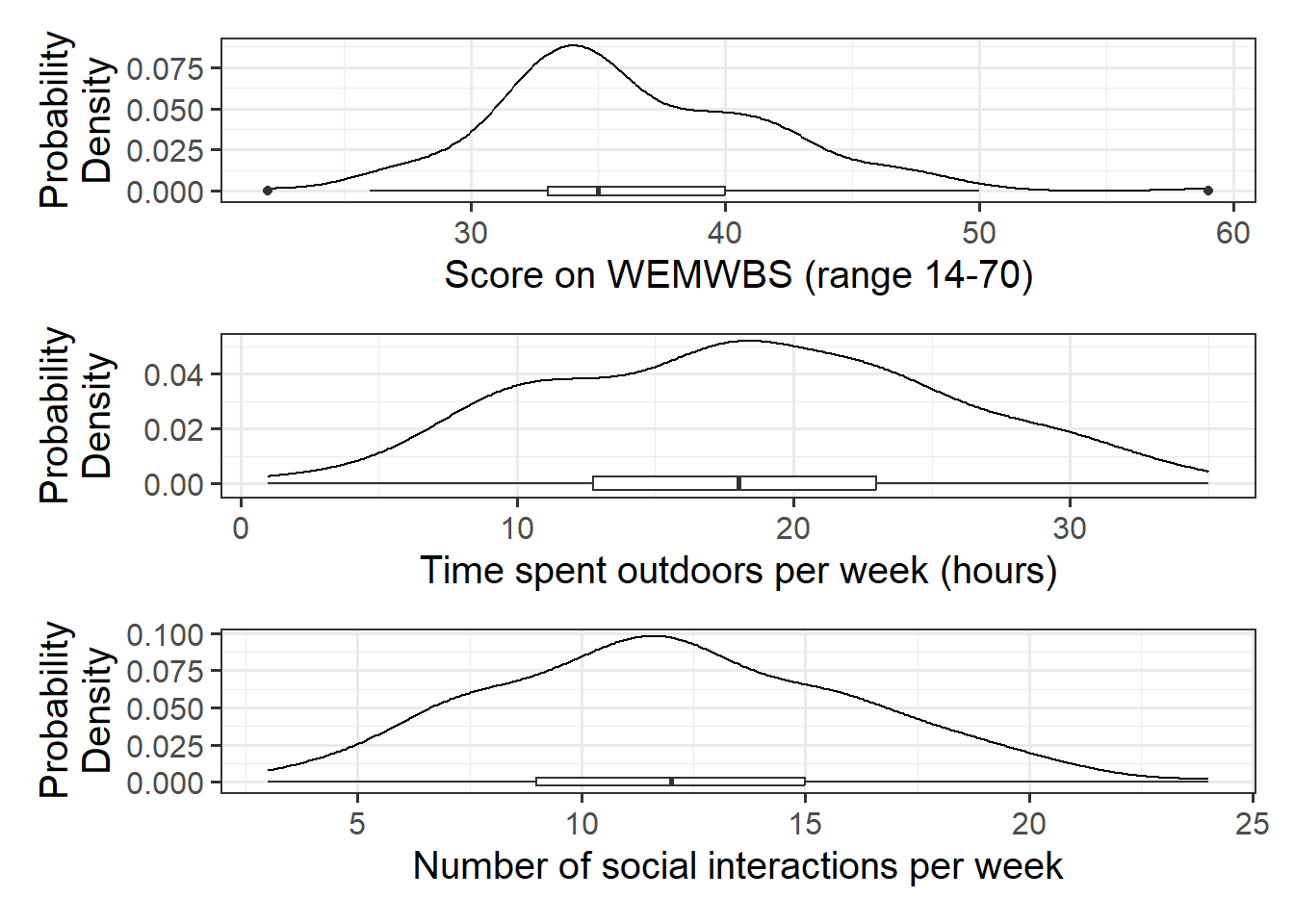
Alongside descriptive statistics, visualize the marginal distributions of the wellbeing, outdoor_time, and social_int variables.

Hint

Plot interpretation
- The shape, center and spread of the distribution - Whether the distribution is symmetric or skewed - Whether the distribution is unimodal or bimodal

Plotting tips
- Use \n to wrap text in your titles and or axis labels - The patchwork package allows us to arrange multiple plots in two ways - | arranges the plots adjacent to one another, and / arranges the plots on top of one another

Table tips
- The kableExtra package allows us to produce well formatted tables for our descriptive statistics. To do so, you need to specify the kable() and kable_styling() arguments

Solution

You should be familiar now with how to visualise a marginal distribution. You might choose histograms, density curves, or boxplots, or a combination:

wellbeing_plot <- 
  ggplot(data = mwdata, aes(x = wellbeing)) +
  geom_density() +
  geom_boxplot(width = 1/200) +
  labs(x = "Score on WEMWBS (range 14-70)", y = "Probability\nDensity")

outdoortime_plot <- 
  ggplot(data = mwdata, aes(x = outdoor_time)) +
  geom_density() +
  geom_boxplot(width = 1/200) +
  labs(x = "Time spent outdoors per week (hours)", y = "Probability\nDensity")

social_plot <- 
  ggplot(data = mwdata, aes(x = social_int)) +
  geom_density() +
  geom_boxplot(width = 1/200) +
  labs(x = "Number of social interactions per week", y = "Probability\nDensity")

# arrange plots vertically 
wellbeing_plot / outdoortime_plot / social_plot

Figure 1: Marginal distribution plots of wellbeing sores, weekly hours spent outdoors, and social interactions

Summary statistics for wellbeing, outdoor time, and social interactions:

descriptives <- mwdata %>% 
  summarize(
    M_Wellbeing = mean(wellbeing), 
    SD_Wellbeing = sd(wellbeing),
    M_OutTime = mean(outdoor_time), 
    SD_OutTime = sd(outdoor_time),
    M_SocInt = mean(social_int), 
    SD_SocInt = sd(social_int)
    )
descriptives

# A tibble: 1 × 6
  M_Wellbeing SD_Wellbeing M_OutTime SD_OutTime M_SocInt SD_SocInt
        <dbl>        <dbl>     <dbl>      <dbl>    <dbl>     <dbl>
1        36.3         5.39      18.3       7.10     12.1      4.02

We can make this into a well formatted table using kable():

kable(descriptives, caption = "Wellbeing, Social Interactions, and Outdoor Time Descriptive Statistics", digits = 2) %>%
        kable_styling()

Wellbeing, Social Interactions, and Outdoor Time Descriptive Statistics

M_Wellbeing	SD_Wellbeing	M_OutTime	SD_OutTime	M_SocInt	SD_SocInt
36.3	5.39	18.25	7.1	12.06	4.02

• The marginal distribution of scores on the WEMWBS was unimodal with a mean of approximately 36.3. There was variation in WEMWBS scores (SD = 5.39)
  
• The marginal distribution of weekly hours spent outdoors was unimodal with a mean of approximately 18.25. There was variation in weekly hours spent outdoors (SD = 7.1)
• The marginal distribution of numbers of social interactions per week was unimodal with a mean of approximately 12.06. There was variation in numbers of social interactions (SD = 4.02)

Question 3

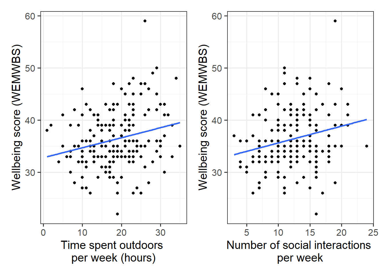
Produce plots of the associations between the outcome variable (wellbeing) and each of the explanatory variables.

Hint

Plot interpretation
- Direction of association - Form of association (can it be summarised well with a straight line?)
- Strength of association (how closely do points fall to a recognizable pattern such as a line?) - Unusual observations that do not fit the pattern of the rest of the observations and which are worth examining in more detail

Plot tips
- use \n to wrap text in your titles and or axis labels - consider using geom_smooth() to superimpose the best-fitting line describing the association of interest

Solution

wellbeing_outdoor <- 
  ggplot(data = mwdata, aes(x = outdoor_time, y = wellbeing)) +
  geom_point() +
  geom_smooth(method = "lm", se = FALSE) + 
  labs(x = "Time spent outdoors \nper week (hours)", y = "Wellbeing score (WEMWBS)")

wellbeing_social <- 
  ggplot(data = mwdata, aes(x = social_int, y = wellbeing)) +
  geom_point() +
  geom_smooth(method = "lm", se = FALSE) + 
  labs(x = "Number of social interactions \nper week", y = "Wellbeing score (WEMWBS)")

# place plots adjacent to one another
wellbeing_outdoor | wellbeing_social

Figure 2: Scatterplots displaying the relationships between scores on the WEMWBS and a) weekly outdoor time (hours), and b) weekly number of social interactions

The scatterplots we created above show weak, positive, and linear associations both between wellbeing and outdoor time, and between wellbeing and the number of weekly social interactions.

Question 4

Produce a correlation matrix of the variables which are to be used in the analysis, and write a short paragraph describing the associations.

Hint

Correlation Matrix
Review Q2 of your Week 1 lab for guidance on how to produce a correlation matrix.

APA Format
Make sure to round your numbers in-line with APA 7th edition guidelines. The round() function will come in handy here, as might this APA numbers and statistics guide!

Solution

We can either:

Index dataframe ([])

# correlation matrix of the three columns of interest (check which columns we need - in this case, 2,3, and 5)
round(cor(mwdata[,c(5,3,2)]), digits = 2)

             wellbeing social_int outdoor_time
wellbeing         1.00       0.24         0.25
social_int        0.24       1.00        -0.04
outdoor_time      0.25      -0.04         1.00

Variable selection (select())

# select only the columns we want by variable name, and pass this to cor()
mwdata %>% 
  select(wellbeing, social_int, outdoor_time) %>%
  cor() %>%
    round(digits = 2)

             wellbeing social_int outdoor_time
wellbeing         1.00       0.24         0.25
social_int        0.24       1.00        -0.04
outdoor_time      0.25      -0.04         1.00

• There was a weak, positive, linear association between WEMWBS scores and weekly outdoor time for the participants in the sample (\(r\) = .25). Higher number of hours spent outdoors each week was associated, on average, with higher wellbeing scores
  
• There was a weak, positive, linear association between WEMWBS scores and the weekly number of social interactions for the participants in the sample (\(r\) = .24). More social interactions were associated, on average, with higher wellbeing scores
• There was a negligible negative correlation between weekly outdoor time and the weekly number of social interactions (\(r\) = -.04)

Model Fitting & Interpretation

Question 5

Recall the model specified in Q1, and:

1. State the parameters of the model. How do we denote parameter estimates?
   
2. Fit the linear model in using lm(), assigning the output to an object called mdl1.

Hint

As we did for simple linear regression, we can fit our multiple regression model using the lm() function. We can add as many explanatory variables as we like, separating them with a +.

model_name <- lm(<response variable> ~ 1 + <explanatory variable 1> + <explanatory variable 2> + ... , data = <dataframe>)

Solution

A model for the association between \(x_1\) = weekly numbers of social interactions, \(x_2\) = weekly outdoor time, and \(y\) = scores on the WEMWBS can be given by: \[ y = \beta_0 + \beta_1 x_1 + \beta_2 x_2 + \epsilon \\ \quad \\ \text{where} \quad \epsilon \sim N(0, \sigma) \text{ independently} \]

In the model specified above,

• \(\mu_{y|x_1, x_2} = \beta_0 + \beta_1 x + \beta_2 x_2\) represents the systematic part of the model giving the mean of \(y\) at each combination of values of \(x_1\) and \(x_2\);
• \(\epsilon\) represents the error (deviation) from that mean, and the errors are independent from one another.

The parameters of our model are:

• \(\beta_0\) (The intercept);
• \(\beta_1\) (The slope across values of \(x_1\));
• \(\beta_2\) (The slope across values of \(x_2\));
  
• \(\sigma\) (The standard deviation of the errors).

When we estimate these parameters from the available data, we have a fitted model (recall that the h\(\hat{\textrm{a}}\)ts are used to distinguish our estimates from the true unknown parameters): \[ \widehat{Wellbeing} = \hat \beta_0 + \hat \beta_1 \cdot Social Interactions + \hat \beta_2 \cdot Outdoor Time \] And we have residuals \(\hat \epsilon = y - \hat y\) which are the deviations from the observed values and our model-predicted responses.

Fitting the model in R:

mdl1 <- lm(wellbeing ~ social_int + outdoor_time, data = mwdata)

Visual

Note that for simple linear regression we talked about our model as a line in 2 dimensions: the systematic part \(\beta_0 + \beta_1 x\) defined a line for \(\mu_y\) across the possible values of \(x\), with \(\epsilon\) as the random deviations from that line. But in multiple regression we have more than two variables making up our model.

In this particular case of three variables (one outcome + two explanatory), we can think of our model as a regression surface (see Figure 3). The systematic part of our model defines the surface across a range of possible values of both \(x_1\) and \(x_2\). Deviations from the surface are determined by the random error component, \(\hat \epsilon\).

Figure 3: Regression surface for wellbeing ~ social_int + outdoor_time, from two different angles

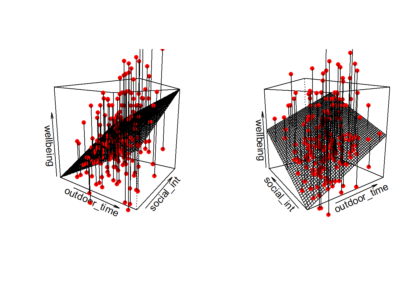
Don’t worry about trying to figure out how to visualise it if we had any more explanatory variables! We can only concieve of 3 spatial dimensions. One could imagine this surface changing over time, which would bring in a 4th dimension, but beyond that, it’s not worth trying!.

Question 6

Using any of:

• mdl1
• mdl1$coefficients
• coef(mdl1)
• coefficients(mdl1)
• summary(mdl1)

Write out the estimated parameter values of:

1. \(\hat \beta_0\), the estimated average wellbeing score associated with zero hours of outdoor time and zero social interactions per week.
   
2. \(\hat \beta_1\), the estimated increase in average wellbeing score associated with an additional social interaction per week (an increase of one), holding weekly outdoor time constant.
   
3. \(\hat \beta_2\), the estimated increase in average wellbeing score associated with one hour increase in weekly outdoor time, holding the number of social interactions constant

Note

Q: What do we mean by hold constant / controlling for / partialling out / residualizing for?

A: When the remaining explanatory variables are held at the same value or are fixed.

Solution

mdl1$coefficients

mdl1$coefficients

 (Intercept)   social_int outdoor_time 
  28.6201808    0.3348821    0.1990943 

coef(mdl1)

coef(mdl1)

 (Intercept)   social_int outdoor_time 
  28.6201808    0.3348821    0.1990943 

coefficients(mdl1)

coefficients(mdl1)

 (Intercept)   social_int outdoor_time 
  28.6201808    0.3348821    0.1990943 

summary(mdl1)

Look under the “Estimate” column:

summary(mdl1)

Call:
lm(formula = wellbeing ~ social_int + outdoor_time, data = mwdata)

Residuals:
     Min       1Q   Median       3Q      Max 
-15.7611  -3.1308  -0.4213   3.3126  18.8406 

Coefficients:
             Estimate Std. Error t value Pr(>|t|)    
(Intercept)  28.62018    1.48786  19.236  < 2e-16 ***
social_int    0.33488    0.08929   3.751 0.000232 ***
outdoor_time  0.19909    0.05060   3.935 0.000115 ***
---
Signif. codes:  0 '***' 0.001 '**' 0.01 '*' 0.05 '.' 0.1 ' ' 1

Residual standard error: 5.065 on 197 degrees of freedom
Multiple R-squared:  0.1265,    Adjusted R-squared:  0.1176 
F-statistic: 14.26 on 2 and 197 DF,  p-value: 1.644e-06

1. \(\hat \beta_0\) = 28.62
   
2. \(\hat \beta_1\) = 0.33
   
3. \(\hat \beta_2\) = 0.2

Question 7

Within what distance from the model predicted values (the regression line) would we expect 95% of WEMWBS wellbeing scores to be?

Hint

Either sigma() or part of the output from summary() will help you here.

Solution

sigma(mdl1)

sigma(mdl1)

[1] 5.065003

summary(mdl1)

Look at the “Residual standard error” entry of the summary(mdl) output:

summary(mdl1)

Call:
lm(formula = wellbeing ~ social_int + outdoor_time, data = mwdata)

Residuals:
     Min       1Q   Median       3Q      Max 
-15.7611  -3.1308  -0.4213   3.3126  18.8406 

Coefficients:
             Estimate Std. Error t value Pr(>|t|)    
(Intercept)  28.62018    1.48786  19.236  < 2e-16 ***
social_int    0.33488    0.08929   3.751 0.000232 ***
outdoor_time  0.19909    0.05060   3.935 0.000115 ***
---
Signif. codes:  0 '***' 0.001 '**' 0.01 '*' 0.05 '.' 0.1 ' ' 1

Residual standard error: 5.065 on 197 degrees of freedom
Multiple R-squared:  0.1265,    Adjusted R-squared:  0.1176 
F-statistic: 14.26 on 2 and 197 DF,  p-value: 1.644e-06

The estimated standard deviation of the errors is \(\hat \sigma\) = 5.07. We would expect 95% of wellbeing scores to be within about 10.13 (\(2 \hat \sigma\)) from the model fit.

Question 8

Based on the model, predict the wellbeing scores for the following individuals:

• Leah: Social Interactions = 25; Outdoor Time = 3
• Sean: Social Interactions = 19; Outdoor Time = 36
• Mike: Social Interactions = 15; Outdoor Time = 20
• Donna: Social Interactions = 7; Outdoor Time = 1

Who has the highest predicted wellbeing score, and who has the lowest?

Solution

First we need to pass the data into R:

wellbeing_query <- tibble(social_int = c(25, 19, 15, 7),
                          outdoor_time = c(3, 36, 20, 1))

And next use predict() to get their estimated wellbeing scores:

predict(mdl1, newdata = wellbeing_query)

       1        2        3        4 
37.58952 42.15034 37.62530 31.16345 

Sean has the highest predicted wellbeing score (42.15), and Donna the lowest (31.16).

Writing Up & Presenting Results

Question 9

Provide key model results in a formatted table.

Solution

tab_model(mdl1,
          dv.labels = "Wellbeing (WEMWBS Scores)",
          pred.labels = c("social_int" = "Social Interactions (number per week)",
                          "outdoor_time" = "Outdoor Time (hours per week)"),
          title = "Regression Table for Wellbeing Model")

Table 1: Regression Table for Wellbeing Model

	Wellbeing (WEMWBS Scores)
Predictors	Estimates	CI	p
(Intercept)	28.62	25.69 – 31.55	<0.001
Social Interactions (number per week)	0.33	0.16 – 0.51	<0.001
Outdoor Time (hours per week)	0.20	0.10 – 0.30	<0.001
Observations	200
R2 / R2 adjusted	0.126 / 0.118

Question 10

Interpret your results in the context of the research question.

Make reference to the your regression table.

Hint

Make sure to include a decision in relation to your null hypothesis - based on the evidence, should you reject or fail to reject the null?

Solution

A multiple regression model was used to determine if there was an association between well-being and time spent outdoors after taking into account the association between well-being and social interactions. As presented in Table 1, outdoor time was significantly associated with wellbeing scores \((\beta = 0.20, SE = 0.05, p < .001)\) after controlling for the number of weekly social interactions. Results suggested that for every additional hour spent outdoors each week, wellbeing scores increased by 0.20 points. Therefore, we should reject the null hypothesis since \(p < .05\).