Simple Linear Regression

Learning Objectives

At the end of this lab, you will:

1. Be able to specify a simple linear model.
2. Understand what fitted values and residuals are.
3. Be able to interpret the coefficients of a fitted model.

Requirements

1. Be up to date with lectures from Weeks 1 & 2
2. Have completed Week 1 lab exercises

Required R Packages

Remember to load all packages within a code chunk at the start of your RMarkdown file using library(). If you do not have a package and need to install, do so within the console using install.packages(" "). For further guidance on installing/updating packages, see Section C here.

For this lab, you will need to load the following package(s):

• tidyverse
• sjPlot

Lab Data

You can download the data required for this lab here or read it in via this link https://uoepsy.github.io/data/riverview.csv.

Study Overview

Research Question

Is there an overall effect of the number of social interactions on wellbeing scores?

Wellbeing/Rurality data codebook.

Description

From the Edinburgh & Lothians, 100 city/suburb residences and 100 rural residences were chosen at random and contacted to participate in the study. The Warwick-Edinburgh Mental Wellbeing Scale (WEMWBS), was used to measure mental health and well-being.

Participants filled out a questionnaire including items concerning: estimated average number of hours spent outdoors each week, estimated average number of social interactions each week (whether on-line or in-person), whether a daily routine is followed (yes/no). For those respondents who had an activity tracker app or smart watch, they were asked to provide their average weekly number of steps.

The data in wellbeing.csv contain seven attributes collected from a random sample of \(n=200\) hypothetical residents over Edinburgh & Lothians, and include:

• wellbeing: Warwick-Edinburgh Mental Wellbeing Scale (WEMWBS), a self-report measure of mental health and well-being. The scale is scored by summing responses to each item, with items answered on a 1 to 5 Likert scale. The minimum scale score is 14 and the maximum is 70.
  
• outdoor_time: Self report estimated number of hours per week spent outdoors
  
• social_int: Self report estimated number of social interactions per week (both online and in-person)
• routine: Binary 1=Yes/0=No response to the question “Do you follow a daily routine throughout the week?”
• location: Location of primary residence (City, Suburb, Rural)
• steps_k: Average weekly number of steps in thousands (as given by activity tracker if available)
• age: Age in years of respondent

Preview

The first six rows of the data are:

age	outdoor_time	social_int	routine	wellbeing	location	steps_k
28	12	13	1	36	rural	21.6
56	5	15	1	41	rural	12.3
25	19	11	1	35	rural	49.8
60	25	15	0	35	rural	NA
19	9	18	1	32	rural	48.1
34	18	13	1	34	rural	67.3

Setup

Setup

1. Create a new RMarkdown file
2. Load the required package(s)
3. Read the wellbeing dataset into R, assigning it to an object named mwdata

Solution

#Loading the required package(s)
library(tidyverse)
library(sjPlot)

# Reading in data and storing to an object named 'mwdata'
mwdata <- read_csv("https://uoepsy.github.io/data/wellbeing_rural.csv")

Exercises

Data Exploration

The common first port of call for almost any statistical analysis is to explore the data, and we can do this visually and/or numerically.

================ Description	Marginal Distributions | Bivariate Associations | =================================================================================================================================================================+==============================================================================================================================================================================+ The distribution of each variable without reference to the values of the other variables | Describing the relationship between two numeric variables |
Visually	Plot each variable individually. You could use, for example, geom_density() for a density plot or geom_histogram() for a histogram to comment on and/or examine: The shape of the distribution. Look at the shape, centre and spread of the distribution. Is it symmetric or skewed? Is it unimodal or bimodal? Identify any unusual observations. Do you notice any extreme observations (i.e., outliers)?	Plot associations among two variables. | | | You could use, for example, geom_point() for a scatterplot to comment on and/or examine: | | The direction of the association indicates whether there is a positive or negative association The form of association refers to whether the relationship between the variables can be summarized well with a straight line or some more complicated pattern The strength of association entails how closely the points fall to a recognizable pattern such as a line Unusual observations that do not fit the pattern of the rest of the observations and which are worth examining in more detail
Numerically	Compute and report summary statistics e.g., mean, standard deviation, median, min, max, etc. You could, for example, calculate summary statistics such as the mean (mean()) and standard deviation (sd()), etc. within summarize()	Compute and report the correlation coefficient. You can use the cor() function to calculate this

Marginal Distributions

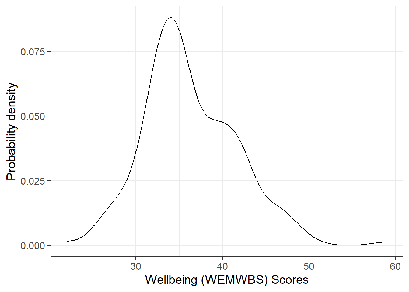
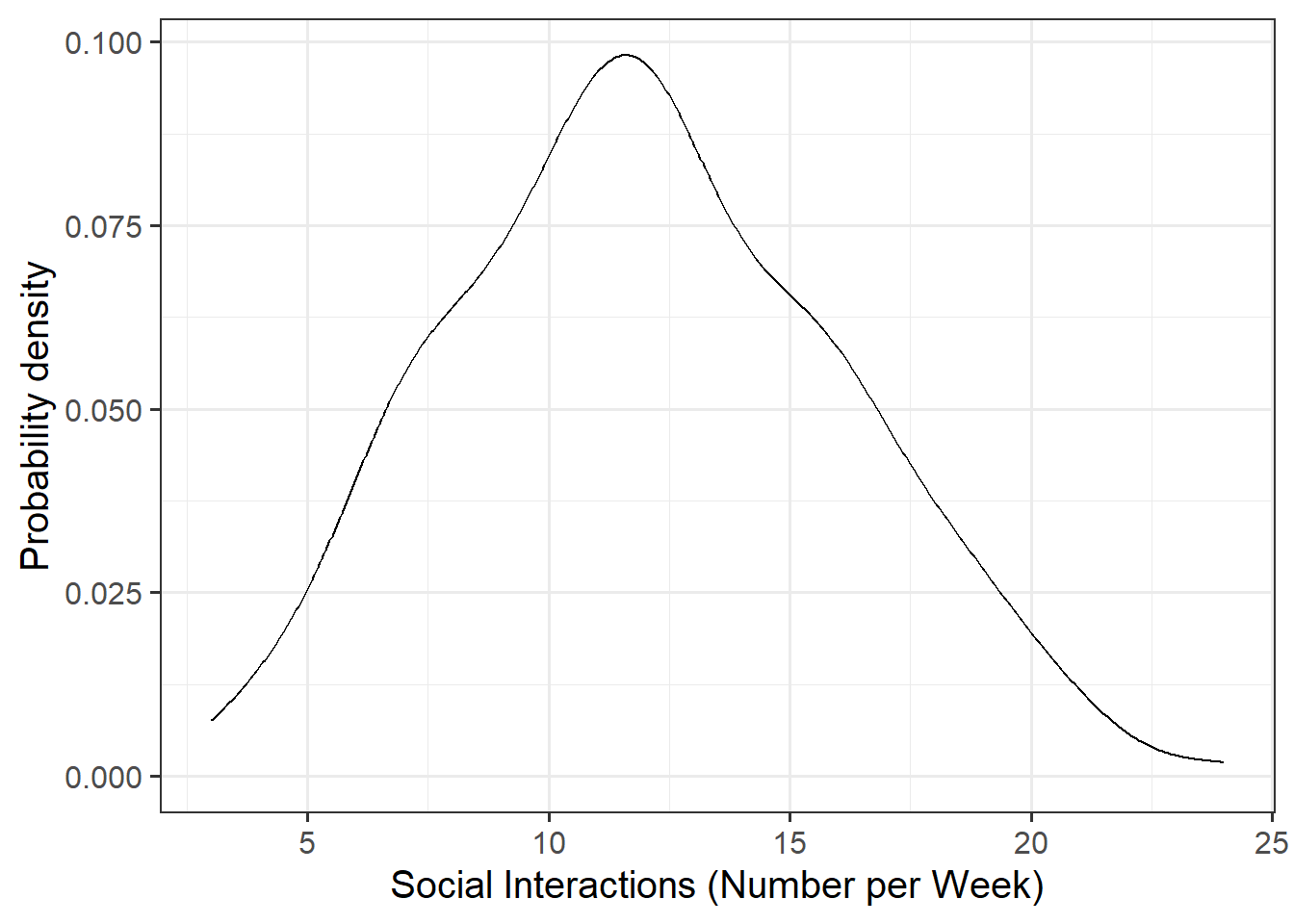
Question 1

Visualise and describe the marginal distributions of wellbeing scores and social interactions.

Solution

Wellbeing (WEMWBS) Scores

Visualisation of distribution:

ggplot(data = mwdata, aes(x = wellbeing)) +
  geom_density() +
  labs(x = "Wellbeing (WEMWBS) Scores", 
       y = "Probability density")

Figure 1: Distribution of Wellbeing (WEMWBS) Scores

Initial observations from plot:

• The distribution of wellbeing scores was unimodal
• Most of the wellbeing scores were between roughly 30 and 45
• The lowest wellbeing in the sample was approximately 22 and the highest approximately 59. This suggested there was a fair high degree of variation in the data
• Scores were within the range of possible values

Descriptive (or summary) statistics for wellbeing scores:

desc_wellbeing <- mwdata %>% 
  summarize(
    M = mean(wellbeing), 
    SD = sd(wellbeing)
    )
desc_wellbeing

# A tibble: 1 × 2
      M    SD
  <dbl> <dbl>
1  36.3  5.39

Following the exploration above, we can describe the wellbeing variable as follows:

The marginal distribution of scores on the WEMWBS was unimodal with a mean of approximately 36.3. There was variation in WEMWBS scores (SD = 5.39)

Social Interactions

Visualisation of distribution:

ggplot(data = mwdata, aes(x = social_int)) +
  geom_density() +
  labs(x = "Social Interactions (Number per Week)", 
       y = "Probability density")

Figure 2: Distribution of Number of Social Interactions

Initial observations from plot:

• The distribution of social interactions was unimodal
• Most of the participants had between 8 and 15 social interactions per week
• The fewest social interactions per week was approximately 3, and the highest approximately 24. This suggested there was a fair high degree of variation in the data

Descriptive (or summary) statistics for the number of weekly social interactions per week:

desc_social <- mwdata %>% 
  summarize(
    M = mean(social_int), 
    SD = sd(social_int)
    )
desc_social

# A tibble: 1 × 2
      M    SD
  <dbl> <dbl>
1  12.1  4.02

Following the exploration above, we can describe the social interactions variable as follows:

The marginal distribution of numbers of social interactions per week was unimodal with a mean of approximately 12.06. There was variation in numbers of social interactions (SD = 4.02)

Associations among Variables

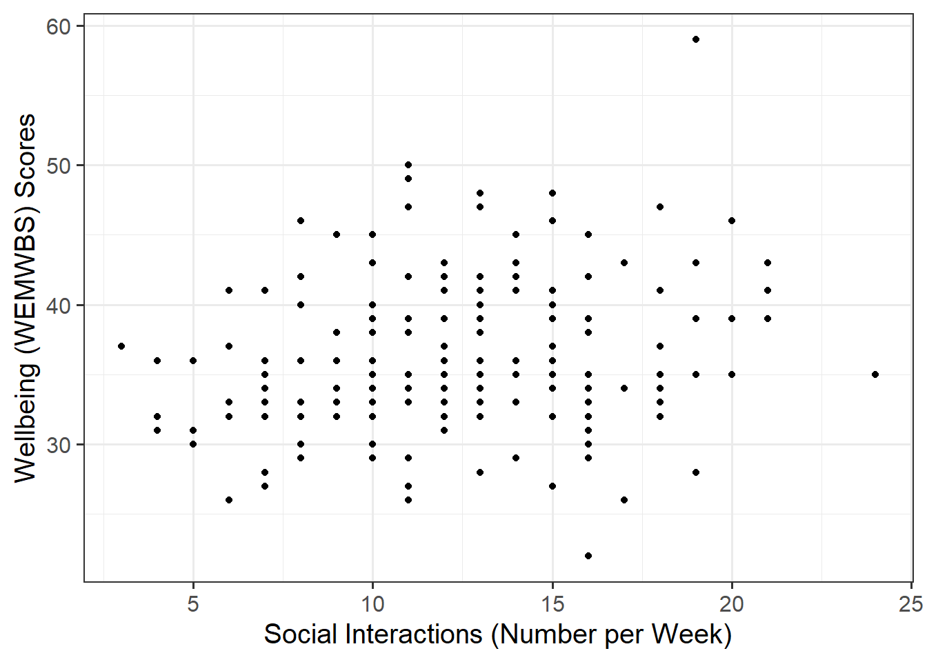
Question 2

Create a scatterplot of wellbeing score and social interactions before calculating the correlation between them.

Correlation Matrix

A table showing the correlation coefficients - \(r_{(x,y)}=\frac{\mathrm{cov}(x,y)}{s_xs_y}\) - between variables. Each cell in the table shows the association between two variables. The diagonals show the correlation of a variable with itself (and are therefore always equal to 1).

In R, we can create a correlation matrix by giving the cor() function a dataframe. However, we only want to give it 2 columns here. Think about how we select specific columns, either giving the column numbers inside [], or using select().

Making reference to both the plot and correlation coefficient, describe the association between wellbeing and social interactions among participants in the Edinburgh & Lothians sample.

Hint

Plot
We are trying to investigate how wellbeing varies by varying numbers of weekly social interactions. Hence, wellbeing is the dependent variable (on the y-axis), and social interactions is the independent variable (on the x-axis).

Correlation
Make sure to round your numbers in-line with APA 7th edition guidelines. The round() function will come in handy here, as might this APA numbers and statistics guide!

Solution

Let’s produce a scatterplot:

ggplot(data = mwdata, aes(x = social_int, y = wellbeing)) +
  geom_point() +
  labs(x = "Social Interactions (Number per Week)", 
       y = "Wellbeing (WEMWBS) Scores")

Figure 3: Association between Wellbeing and Social Interactions

To comment on the strength of the linear association we compute the correlation coefficient in either of the following ways:

Indexing ([])

# correlation matrix of the two columns of interest - 3 & 5
round(cor(mwdata[,c(3,5)]), digits = 2)

           social_int wellbeing
social_int       1.00      0.24
wellbeing        0.24      1.00

Selection (select())

# select only the columns we want by name, and pass this to cor()
mwdata %>% 
  select(social_int, wellbeing) %>%
  cor() %>%
    round(digits = 2)

           social_int wellbeing
social_int       1.00      0.24
wellbeing        0.24      1.00

And we can see that via either method, the correlation is \[ r_{\text({Social~Interactions,~~ Wellbeing})} = .24 \]

There was a weak, positive, linear association between the weekly number of social interactions and WEMWBS scores for the participants in the sample (\(r\) = .24). More social interactions were associated, on average, with higher wellbeing scores.

Model Specification and Fitting

The scatterplot highlighted a linear relationship, where the data points were scattered around an underlying linear pattern with a roughly-constant spread as x varied.

Hence, we will try to fit a simple (i.e., one x variable only) linear regression model:

\[ y_i = \beta_0 + \beta_1 x_i + \epsilon_i \\ \quad \text{where} \quad \epsilon_i \sim N(0, \sigma) \text{ independently} \]

What does \(y_i = \beta_0 + \beta_1 x_i + \epsilon_i \quad \text{where} \quad \epsilon_i \sim N(0, \sigma) \text{ independently}\) mean?

Lets break the statement down into smaller parts:

\(y_i = \beta_0 + \beta_1 x_i + \epsilon_i\)

• \(y_i\) is our measured outcome variable (our DV)
• \(x_i\) is our measured predictor variable (our IV)
• \(\beta_0\) is the model intercept
• \(\beta_1\) is the model slope

\(\epsilon \sim N(0, \sigma) \text{ independently}\)

• \(\epsilon\) is the residual error
• \(\sim\) means ‘distributed according to’
• \(\sim N(0, \sigma) \text{ independently}\) means ‘normal distribution with a mean of 0 and a variance of \(\sigma\)’
• Together, we can say that the errors around the line have a mean of zero and constant spread as x varies.

Question 3

First, write the equation of the fitted line.

Next, using the lm() function, fit a simple linear model to predict wellbeing (DV) by social interactions (IV), naming the output mdl.

Lastly, update your equation of the fitted line to include the estimated coefficients.

Hint

The syntax of the lm() function is:

[model name] <- lm([response variable i.e., dependent variable] ~ [explanatory variable i.e., independent variable], data = [dataframe])

Solution

First, lets specify the fitted model, which can be written either as:

Option A

\[ \widehat{Wellbeing} = \hat \beta_0 + \hat \beta_1 \cdot Social~Interactions \]

Option B

\[ \widehat{Wellbeing} = \hat \beta_0 \cdot 1 + \hat \beta_1 \cdot Social~Interactions \]

To fit the model in R, as the variables are in the mwdata dataframe, we would write:

Option A

mdl <- lm(wellbeing ~ social_int, data = mwdata)
mdl

Call:
lm(formula = wellbeing ~ social_int, data = mwdata)

Coefficients:
(Intercept)   social_int  
    32.4077       0.3222  

Option B

mdl <- lm(wellbeing ~ 1 + social_int, data = mwdata)
mdl

Call:
lm(formula = wellbeing ~ 1 + social_int, data = mwdata)

Coefficients:
(Intercept)   social_int  
    32.4077       0.3222  

Why is there a 1 in the Option B’s?

When we specify the linear model in R, we include after the tilde sign (\(\sim\)), the variables that appear to the right of the \(\hat \beta\)s. The intercept, or \(\beta_0\), is a constant. That is, we could write it as multiplied by 1.

Including the 1 explicitly is not necessary because it is included by default (you can check this by comparing the outputs of A & B above with and without the 1 included - the estimates are the same!). After a while, you will find you just want to drop the 1 (i.e., Option B) when calling lm() because you know that it’s going to be there, but in these early weeks we tried to keep it explicit to make it clear that you want to the intercept to be estimated.

Note that by calling the name of the fitted model, mdl, you can see the estimated regression coefficients \(\hat \beta_0\) and \(\hat \beta_1\). We can add these values to the fitted line:

\[ \widehat{Wellbeing} = 32.41 + 0.32 \cdot Social~Interactions \\ \]

Question 4

Explore the following equivalent ways to obtain the estimated regression coefficients — that is, \(\hat \beta_0\) and \(\hat \beta_1\) — from the fitted model:

• mdl
• mdl$coefficients
• coef(mdl)
• coefficients(mdl)
• summary(mdl)

Solution

The estimated parameters returned by the below methods are all equivalent. However, summary() returns more information.

mdl()

Simply invoke the name of the fitted model:

mdl

Call:
lm(formula = wellbeing ~ 1 + social_int, data = mwdata)

Coefficients:
(Intercept)   social_int  
    32.4077       0.3222  

mdl$coefficients

mdl$coefficients

(Intercept)  social_int 
 32.4077070   0.3221959 

coef(mdl)

coef(mdl)

(Intercept)  social_int 
 32.4077070   0.3221959 

coefficients(mdl)

coefficients(mdl)

(Intercept)  social_int 
 32.4077070   0.3221959 

summary(mdl)

Look under the “Estimate” column:

summary(mdl)

Call:
lm(formula = wellbeing ~ 1 + social_int, data = mwdata)

Residuals:
     Min       1Q   Median       3Q      Max 
-15.5628  -3.2741  -0.7908   3.3703  20.4706 

Coefficients:
            Estimate Std. Error t value Pr(>|t|)    
(Intercept) 32.40771    1.17532  27.573  < 2e-16 ***
social_int   0.32220    0.09243   3.486 0.000605 ***
---
Signif. codes:  0 '***' 0.001 '**' 0.01 '*' 0.05 '.' 0.1 ' ' 1

Residual standard error: 5.247 on 198 degrees of freedom
Multiple R-squared:  0.05781,   Adjusted R-squared:  0.05306 
F-statistic: 12.15 on 1 and 198 DF,  p-value: 0.0006045

The estimated intercept is \(\hat \beta_0 = 32.41\) and the estimated slope is \(\hat \beta_1 = 0.32\).

Question 5

Explore the following equivalent ways to obtain the estimated standard deviation of the errors — that is, \(\hat \sigma\) — from the fitted model mdl:

• sigma(mdl)
• summary(mdl)

Huh? What is \(\sigma\)?

The standard deviation of the errors, denoted by \(\sigma\), is an important quantity that our model estimates. It represents how much individual data points tend to deviate above and below the regression line.

A small \(\sigma\) indicates that the points hug the line closely and we should expect fairly accurate predictions, while a large \(\sigma\) suggests that, even if we estimate the line perfectly, we can expect individual values to deviate from it by substantial amounts.

The estimated standard deviation of the errors is denoted \(\hat \sigma\), and is estimated by essentially averaging squared residuals (giving the variance) and taking the square-root:

\[ \begin{align} & \hat \sigma = \sqrt{\frac{SS_{Residual}}{n - k - 1}} \\ \qquad \\ & \text{where} \\ & SS_{Residual} = \textrm{Sum of Squared Residuals} = \sum_{i=1}^n{(\epsilon_i)^2} \end{align} \]

Solution

The estimated standard deviation of the errors can be equivalently obtained by the below methods. However, summary() returns more information.

sigma(mdl)

sigma(mdl)

[1] 5.246982

summary(mdl)

Look at the “Residual standard error” entry of the summary(mdl) output:

summary(mdl)

Call:
lm(formula = wellbeing ~ 1 + social_int, data = mwdata)

Residuals:
     Min       1Q   Median       3Q      Max 
-15.5628  -3.2741  -0.7908   3.3703  20.4706 

Coefficients:
            Estimate Std. Error t value Pr(>|t|)    
(Intercept) 32.40771    1.17532  27.573  < 2e-16 ***
social_int   0.32220    0.09243   3.486 0.000605 ***
---
Signif. codes:  0 '***' 0.001 '**' 0.01 '*' 0.05 '.' 0.1 ' ' 1

Residual standard error: 5.247 on 198 degrees of freedom
Multiple R-squared:  0.05781,   Adjusted R-squared:  0.05306 
F-statistic: 12.15 on 1 and 198 DF,  p-value: 0.0006045

Note

The term “Residual standard error” is a misnomer, as the help page for sigma says (check ?sigma). However, it’s hard to get rid of this bad name as it has been used in too many books showing R output.

The estimated standard deviation of the errors is \(\hat \sigma = 5.25\).

Question 6

Interpret the estimated intercept, slope, and standard deviation of the errors in the context of the research question.

Hint

To interpret the estimated standard deviation of the errors we can use the fact that about 95% of values from a normal distribution fall within two standard deviations of the center.

Solution

Intercept

The estimated wellbeing score associated to zero weekly social interactions is 32.41.

Slope

The estimated increase in wellbeing associated to one additional weekly social interaction is 0.32.

Standard deviation of the errors

For any particular numnber of weekly social interactions, participants’ wellbeing scores should be distributed above and below the regression line with standard deviation estimated to be \(\hat \sigma = 5.25\). Since \(2 \hat \sigma = 10.49\), we expect most (about 95%) of the participants’ wellbeing scores to be within about 11 points from the regression line.

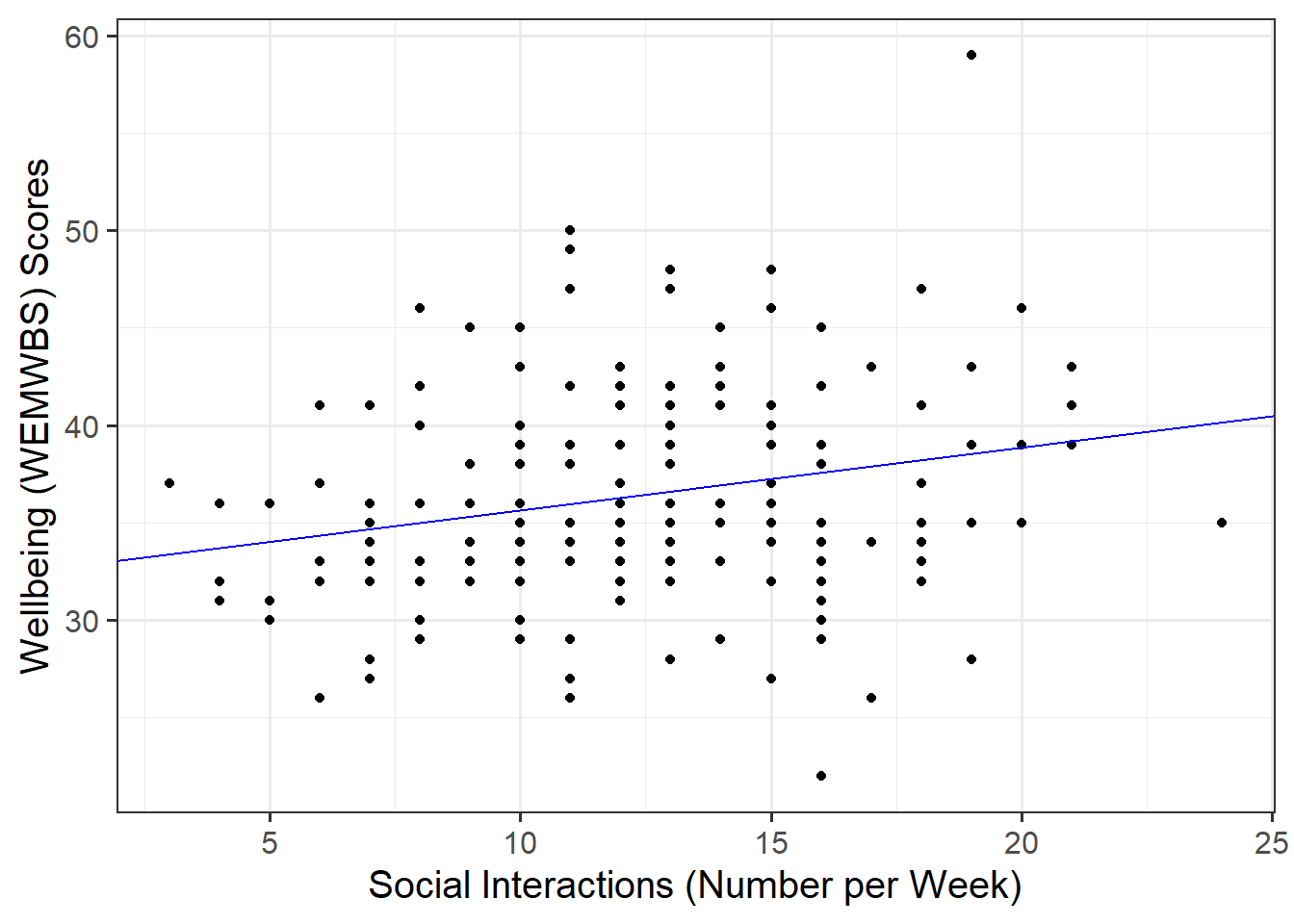
Question 7

Plot the data and the fitted regression line. To do so:

• Extract the estimated regression coefficients e.g., via betas <- coef(mdl)
• Extract the first entry of betas (i.e., the intercept) via betas[1]
• Extract the second entry of betas (i.e., the slope) via betas[2]
• Provide the intercept and slope to the function

Hint

Extracting values
The function coef(mdl) returns a vector (a sequence of numbers all of the same type). To get the first element of the sequence you append [1], and [2] for the second.

Plotting
In your ggplot(), you will need to specify geom_abline(). This might help get you started:

geom_abline(intercept = <intercept>, slope = <slope>)

Solution

First extract the values required:

betas <- coef(mdl)
intercept <- betas[1]
slope <- betas[2]

We can plot the model as follows:

ggplot(data = mwdata, aes(x = social_int, y = wellbeing)) +
  geom_point() +
  geom_abline(intercept = intercept, slope = slope, color = 'blue') + 
  labs(x = "Social Interactions (Number per Week)", y = "Wellbeing (WEMWBS) Scores")

Predicted Values & Residuals

Predicted Values

Model predicted values for sample data:

We can get out the model predicted values for \(y\), the “y hats” (\(\hat y\)), for the data in the sample using various functions:

• predict(<fitted model>)
• fitted(<fitted model>)
• fitted.values(<fitted model>)
• mdl$fitted.values

For example, this will give us the estimated wellbeing score (point on our regression line) for each observed value of social interactions for each of our 200 participants.

predict(mdl)

       1        2        3        4        5        6        7        8 
36.59625 37.24064 35.95186 37.24064 38.20723 36.59625 38.52943 36.27406 
       9       10       11       12       13       14       15       16 
36.59625 37.24064 34.66308 35.62967 34.66308 36.27406 36.91845 37.88504 
      17       18       19       20       21       22       23       24 
37.56284 37.56284 35.62967 35.30747 35.62967 38.20723 36.27406 35.30747 
      25       26       27       28       29       30       31       32 
38.52943 38.52943 37.56284 36.27406 37.56284 35.30747 37.56284 36.91845 
      33       34       35       36       37       38       39       40 
37.56284 34.34088 37.56284 36.27406 36.27406 36.91845 38.85162 35.30747 
      41       42       43       44       45       46       47       48 
38.20723 36.59625 37.56284 36.27406 36.27406 35.95186 34.34088 38.85162 
      49       50       51       52       53       54       55       56 
35.62967 37.24064 35.62967 34.98527 37.56284 37.24064 34.01869 35.95186 
      57       58       59       60       61       62       63       64 
34.66308 37.88504 36.91845 34.66308 37.88504 35.95186 36.27406 35.95186 
      65       66       67       68       69       70       71       72 
36.27406 36.91845 38.20723 34.01869 35.30747 35.30747 34.66308 39.17382 
      73       74       75       76       77       78       79       80 
34.01869 35.30747 33.69649 38.52943 35.62967 37.56284 39.17382 36.91845 
      81       82       83       84       85       86       87       88 
34.98527 35.95186 36.59625 36.27406 34.66308 35.95186 37.24064 37.88504 
      89       90       91       92       93       94       95       96 
35.62967 37.56284 34.66308 34.66308 37.24064 35.95186 34.98527 35.62967 
      97       98       99      100      101      102      103      104 
35.95186 34.66308 37.24064 35.95186 34.34088 34.66308 37.56284 34.98527 
     105      106      107      108      109      110      111      112 
36.27406 37.88504 39.17382 37.24064 38.52943 35.30747 35.62967 35.95186 
     113      114      115      116      117      118      119      120 
37.24064 36.27406 36.27406 36.59625 36.27406 35.95186 36.59625 35.95186 
     121      122      123      124      125      126      127      128 
37.56284 36.91845 34.34088 34.66308 34.98527 35.95186 34.01869 35.62967 
     129      130      131      132      133      134      135      136 
34.98527 35.62967 33.69649 38.20723 38.20723 35.30747 34.66308 37.56284 
     137      138      139      140      141      142      143      144 
36.91845 35.62967 36.91845 38.52943 36.91845 35.30747 35.62967 37.88504 
     145      146      147      148      149      150      151      152 
36.27406 34.98527 35.30747 36.91845 36.59625 36.59625 35.95186 34.34088 
     153      154      155      156      157      158      159      160 
36.59625 36.59625 34.66308 36.91845 36.27406 35.30747 33.69649 35.62967 
     161      162      163      164      165      166      167      168 
36.27406 37.24064 35.95186 36.59625 33.37429 36.59625 38.20723 36.27406 
     169      170      171      172      173      174      175      176 
38.85162 34.66308 37.24064 35.62967 38.20723 36.27406 36.59625 40.14041 
     177      178      179      180      181      182      183      184 
35.30747 34.98527 34.34088 35.95186 36.59625 34.98527 34.98527 35.62967 
     185      186      187      188      189      190      191      192 
34.66308 34.98527 36.27406 37.88504 36.27406 35.95186 35.95186 36.59625 
     193      194      195      196      197      198      199      200 
37.56284 36.27406 36.27406 35.95186 34.66308 35.62967 36.27406 37.24064 

Model predicted values for other (unobserved) data:

To compute the model-predicted values for unobserved data (i.e., data not contained in the sample), we can use the following function:

• predict(<fitted model>, newdata = <dataframe>)

For this example, we first need to remember that the model predicts wellbeing using the independent variable social_int. Hence, if we want predictions for new (unobserved) data, we first need to create a tibble with a column called social_int containing the number of weekly social interactions for which we want the prediction, and store this as a dataframe.

#Create dataframe 'newdata' containing 2, 25, and 28 weekly social interactions
newdata <- tibble(social_int = c(2, 25, 28))
newdata

# A tibble: 3 × 1
  social_int
       <dbl>
1          2
2         25
3         28

Then we take newdata and add a new column called wellbeing_hat, computed as the prediction from the fitted mdl using the newdata above:

newdata <- newdata %>%
  mutate(
    wellbeing_hat = predict(mdl, newdata = newdata)
  )
newdata

# A tibble: 3 × 2
  social_int wellbeing_hat
       <dbl>         <dbl>
1          2          33.1
2         25          40.5
3         28          41.4

Residuals

The residuals represent the deviations between the actual responses and the predicted responses and can be obtained either as

• mdl$residuals
• resid(mdl)
• residuals(mdl)
• computing them as the difference between the response (\(y_i\)) and the predicted response (\(\hat y_i\))

Question 8

Use predict(mdl) to compute the fitted values and residuals. Mutate the mwdata dataframe to include the fitted values and residuals as extra columns.

Assign to the following symbols the corresponding numerical values:

• \(y_{3}\) (response variable for unit \(i = 3\) in the sample data)
• \(\hat y_{3}\) (fitted value for the third unit)
• \(\hat \epsilon_{5}\) (the residual corresponding to the 5th unit, i.e., \(y_{5} - \hat y_{5}\))

Solution

mwdata_fitted <- mwdata %>%
  mutate(
    wellbeing_hat = predict(mdl),
    resid = wellbeing - wellbeing_hat
  )

head(mwdata_fitted)

# A tibble: 6 × 9
    age outdoor_time social_int routine wellbeing location steps_k wellbeing_hat
  <dbl>        <dbl>      <dbl>   <dbl>     <dbl> <chr>      <dbl>         <dbl>
1    28           12         13       1        36 rural       21.6          36.6
2    56            5         15       1        41 rural       12.3          37.2
3    25           19         11       1        35 rural       49.8          36.0
4    60           25         15       0        35 rural       NA            37.2
5    19            9         18       1        32 rural       48.1          38.2
6    34           18         13       1        34 rural       67.3          36.6
# ℹ 1 more variable: resid <dbl>

• \(y_{3}\) = 35 (see row 3, column 5)
• \(\hat y_{3}\) = 35.95 (see row 3, column 8)
• \(\hat \epsilon_{5} = y_{5} - \hat y_{5}\) = 32 - 38.21 = -6.21 (see row 5, columns 5 and 8)

Question 9

Provide key model results in a formatted table.

Hint

Use tab_model() from the sjPlot package.

You can rename your DV and IV labels by specifying dv.labels and pred.labels. To do so, specify your variable name on the left, and what you would like this to be named in the table on the right.

Solution

tab_model(mdl,
          dv.labels = "Wellbeing (WEMWBS) Scores",
          pred.labels = c("social_int" = "Social Interactions (Number per Week)"),
          title = "Regression Table for Wellbeing Model")

Table 1: Regression Table for Wellbeing Model

	Wellbeing (WEMWBS) Scores
Predictors	Estimates	CI	p
(Intercept)	32.41	30.09 – 34.73	<0.001
Social Interactions (Number per Week)	0.32	0.14 – 0.50	0.001
Observations	200
R2 / R2 adjusted	0.058 / 0.053

Question 10

Describe the design of the study, and the analyses that you undertook. Interpret your results in the context of the research question and report your model results in full.

Make reference to your descriptive plots and/or statistics and regression table.

Hint

Make sure to write your results up following APA guidelines

Solution

The mwdata dataset contained information on 200 hypothetical participants who lived in Edinburgh & Lothians area. Using a between-subjects design, the researchers collected information on participants’ wellbeing, outdoor time (hours per week), social interactions (number per week), routine, location of residence, average weekly steps, and age.

To visualise the marginal distributions of wellbeing and social interactions, density plots were used. To understand the strength of association between the two variables, the correlation coefficient was estimated. To investigate whether there was an association between there was an overall effect of the number of weekly social interactions on wellbeing (WEMWBS) scores, the following simple linear regression model was used:

\[ \text{Wellbeing} = \beta_0 + \beta_1 \cdot \text{Social Interactions} \] From Figure 1 and Figure 2, we can see that both wellbeing \((M = 36.3, SD = 5.39)\) and social interactions \((M = 12.06, SD = 4.02)\) followed unimodal distributions. There was a weak, positive, linear association between WEMWBS scores and the weekly number of social interactions for the participants in the sample (\(r\) = .24).

Full regression results are displayed in Table 1. The estimated wellbeing score with no social interactions per week was 32.41. Each additional social interaction was associated with a 0.32 point increase in wellbeing scores.