W3: T-tests

Intervals again

Question 1

At the end of last week’s exercises, we estimated the mean sleep-quality rating, and computed a confidence interval, using the formula below.

\[ \begin{align} \text{95\% CI: }& \bar x \pm 1.96 \times SE \\ \end{align} \]

Can you use R to show where the 1.96 comes from?

Hints

qnorm! (see the end of Chapter 5 #uncertainty-due-to-sampling)

Solution 1. The 1.96 comes from 95% of the normal distribution falling within 1.96 standard deviations of the mean:

qnorm(c(0.025, 0.975))

[1] -1.959964  1.959964

Question 2

As we learned in Chapter 6 #t-distributions, the sampling distribution of a statistic has heavier tails the smaller the size of the sample it is derived from. In practice, we are better using \(t\)-distributions to construct confidence intervals and perform statistical tests.

The code below creates a dataframe that contains the number of books read by 7 people in 2024.
(Note tibble is just a tidyverse version of data.frame):

bookdata <- 
  tibble(
    person = c("Martin","Umberto","Monica","Emma","Josiah","Dan","Aja"),
    books_read = c(12,19,9,11,8,28,13)
  )

Calculate the mean number of books read in 2024, and construct an appropriate 95% confidence interval.

Solution 2. Here is our estimated average number of books read:

mean(bookdata$books_read)

[1] 14.28571

And our standard error is still \(\frac{s}{\sqrt{n}}\):

sd(bookdata$books_read)/sqrt(nrow(bookdata))

[1] 2.652171

With \(n = 7\) observations, and estimating 1 mean, we are left with \(6\) degrees of freedom.
For our 95% confidence interval, the \(t^*\) in the formula below is obtained via:¹

qt(0.975, df = 6)

[1] 2.446912

Our confidence interval is therefore:
\[ \begin{align} \text{CI} &= \bar{x} \pm t^* \times SE \\ \text{95\% CI} &= 14.286 \pm 2.447 \times 2.652 \\ \text{95\% CI} &= [7.80,\, 20.78] \\ \end{align} \]

Question 3

Will a 90% confidence interval be wider or narrow?
Calculate it and see.

Solution 3. A 90% confidence interval will be narrower:

qt(0.95, df = 6)

[1] 1.94318

\[ \begin{align} \text{CI} &= \bar{x} \pm t^* \times SE \\ \text{90\% CI} &= 14.286 \pm 1.943 \times 2.652 \\ \text{90\% CI} &= [9.13,\, 19.44] \\ \end{align} \]

The intuition behind this is that our level of confidence is inversely related to the width of the interval.

Take it to the extremes:

• I have 100% confidence that the interval \([-Infinity, +Infinity]\) contains the true population mean.
• If I want an narrower interval, then I have to sacrifice confidence. e.g. a 10% CI: \([13.94, 14.63]\)

Imagine playing a game of ringtoss. A person throwing a 2-meter diameter hoop will have much more confidence that they are going to get it over the pole than a person throwing a 10cm diameter ring.

Procrastination Scores

Research Question Do Edinburgh University students report endorsing procrastination less than the norm?

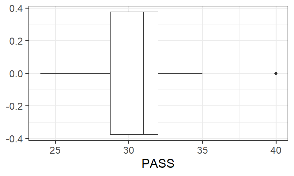
The Procrastination Assessment Scale for Students (PASS) was designed to assess how individuals approach decision situations, specifically the tendency of individuals to postpone decisions (see Solomon & Rothblum, 1984). The PASS assesses the prevalence of procrastination in six areas: writing a paper; studying for an exam; keeping up with reading; administrative tasks; attending meetings; and performing general tasks. For a measure of total endorsement of procrastination, responses to 18 questions (each measured on a 1-5 scale) are summed together, providing a single score for each participant (range 0 to 90). The mean score from Solomon & Rothblum, 1984 was 33.

A student administers the PASS to 20 students from Edinburgh University.
The data are available at https://uoepsy.github.io/data/pass_scores.csv

Question 4

1. Read in the data
2. Calculate some relevant descriptive statistics
3. Check the assumptions that we will be concerned with for a one-sample test of whether the mean PASS scores is less than 33.

Hints

• What counts as “relevant statistics”? Think about the question. It concerns just one variable (the PASS scores), which is numeric. What’s a nice way of describing the center and spread of such a variable?

Solution 4.

Data

pass_scores <- read_csv("https://uoepsy.github.io/data/pass_scores.csv") 
dim(pass_scores)

[1] 20  3

head(pass_scores)

# A tibble: 6 × 3
  sid   school       PASS
  <chr> <chr>       <dbl>
1 s_1   GeoSciences    31
2 s_2   ECA            24
3 s_3   LAW            32
4 s_4   ECA            40
5 s_5   LAW            28
6 s_6   SSPS           31

Descriptives

pass_scores |>
  summarise(
    mPASS = mean(PASS),
    sdPASS = sd(PASS),
    n = n()
  )

# A tibble: 1 × 3
  mPASS sdPASS     n
  <dbl>  <dbl> <int>
1  30.7   3.31    20

Assumptions

We want to check that the data are close to normally distributed. This is especially relevant as we have only 20 datapoints here. The plot below makes it look like we may have one or two data points in the tails of the distribution that are further than we might expect.

ggplot(pass_scores, aes(sample = PASS)) + 
  geom_qq() + 
  geom_qq_line()

But the Shapiro-Wilk test of \(p > .05\) indicates that we are probably okay to continue with our t-test

shapiro.test(pass_scores$PASS)

    Shapiro-Wilk normality test

data:  pass_scores$PASS
W = 0.93617, p-value = 0.2028

Question 5

Our test here is going to have the following hypotheses:

• Null: mean PASS score in Edinburgh Uni students is \(\geq 33\)
• Alternative: mean PASS score in Edinburgh Uni students is \(< 33\)

Manually calculate the relevant test statistic.
Note, we’re doing this manually right now as it’s a useful learning process. In later questions we will switch to the easy way!

Hints

• you can see the step-by-step calculation of a one sample t-test in Chapter 6 #one-sample-t-test.
• The relevant formula is:
  \[ \begin{align} & t = \frac{\bar x - \mu_0}{\frac{s}{\sqrt{n}}} \\ \qquad \\ & \text{Where:} \\ & \bar x : \text{mean of PASS in our sample} \\ & \mu_0 : \text{hypothesised mean score of 33} \\ & s : \text{standard deviation of PASS in our sample} \\ & n : \text{number of observations} \end{align} \]

Solution 5.

pass_scores <- read_csv("https://uoepsy.github.io/data/pass_scores.csv") 

pass_scores |> 
  summarise(
    xbar = mean(PASS),
    s = sd(PASS),
    n = n(),
    t = (xbar - 33)/(s / sqrt(n))
  )

# A tibble: 1 × 4
   xbar     s     n     t
  <dbl> <dbl> <int> <dbl>
1  30.7  3.31    20 -3.11

Question 6

Using the test statistic calculated in question above, compute the p-value.

Hints

• this will be needing the pt() function.
• the degrees of freedom is \(n-1\) (we used one up by estimating the mean).
• The test we are performing is against the null hypothesis that the mean is \(\geq 33\). Our t-statistic is in the broad sense calculated as “mean minus 33”, so negative numbers mean we have a mean lower than 33. These are the instances that we will reject the null hypothesis - if we get a test statistic very low. So we want the lower.tail of the distribution for our p-value.

Solution 6. We have 20 participants, so \(df=19\)

pt(-3.107272, df = 19, lower.tail = TRUE)

[1] 0.002900159

Question 7

Now using the t.test() function, conduct the same test. Check that the numbers match with your step-by-step calculations in the previous two questions.

Hints

Check out the help page for t.test() - there is an argument in the function that allows us to easily change between whether our alternative hypothesis is “less than”, “greater than” or “not equal to”.

Solution 7.

t.test(pass_scores$PASS, mu = 33, alternative = "less")

    One Sample t-test

data:  pass_scores$PASS
t = -3.1073, df = 19, p-value = 0.0029
alternative hypothesis: true mean is less than 33
95 percent confidence interval:
    -Inf 31.9799
sample estimates:
mean of x 
     30.7 

The \(t\) statistic, our \(df\), and our \(p\)-value all match the calculations from the previous questions.

The simple t.test() approach even gives us a confidence interval! Well.. half of one! This is because we conducted a one-sided test. Remember that null hypothesis significance testing is like asking “does our confidence interval contain zero?”. With a one-sided test we only reject the null hypothesis if the test statistic is large in one direction, and so our confidence interval is one-sided also.

Question 8

Create a visualisation to illustrate the results.

Solution 8.

ggplot(data = pass_scores, aes(x=PASS)) + 
  geom_boxplot() + 
  geom_vline(xintercept=33, lty="dashed", col="red")

Figure 1: Distribution of scores on the Procrastination Assessment Scale for Students (PASS) measure. The majority of the sample scored below the suggested normal score of 33 (red dashed line).

Question 9

Write up the results.

Hints

There are some quick example write-ups for each test in Chapter 6 #basic-tests

Solution 9.

A one-sided one-sample t-test was conducted in order to determine if the average score on the Procrastination Assessment Scale for Students (PASS) for a sample of 20 students at Edinburgh University was significantly lower (\(\alpha = .05\)) than the average score of 33 obtained during development of the PASS.

Edinburgh University students scored lower (Mean = 30.7, SD = 3.31) than the score reported by the authors of the PASS (Mean = 33). This difference was statistically significant (\(t(19)=-3.11\), \(p < .05\), one-tailed).

Heights

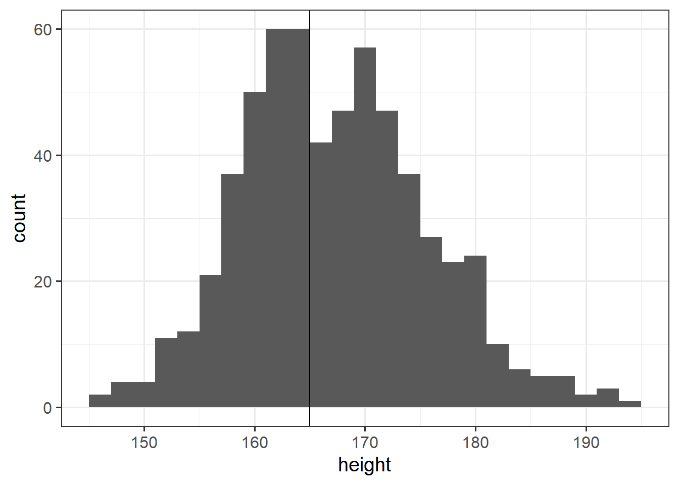
Research Question Is the average height of University of Edinburgh Psychology students different from 165cm?

Data: Past Surveys
In the last few years, we have asked students of the statistics courses in the Psychology department to fill out a little survey.
Anonymised data are available at https://uoepsy.github.io/data/usmr25survey_historical.csv

Note: this does not contain the responses from this year.

surveydata <- 
  read_csv("https://uoepsy.github.io/data/usmr25survey_historical.csv")

Question 10

No more manual calculations of test statistics and p-values for this week.

Conduct a one sample \(t\)-test to evaluate whether the average height of UoE psychology students in the last few years was different from 165cm.

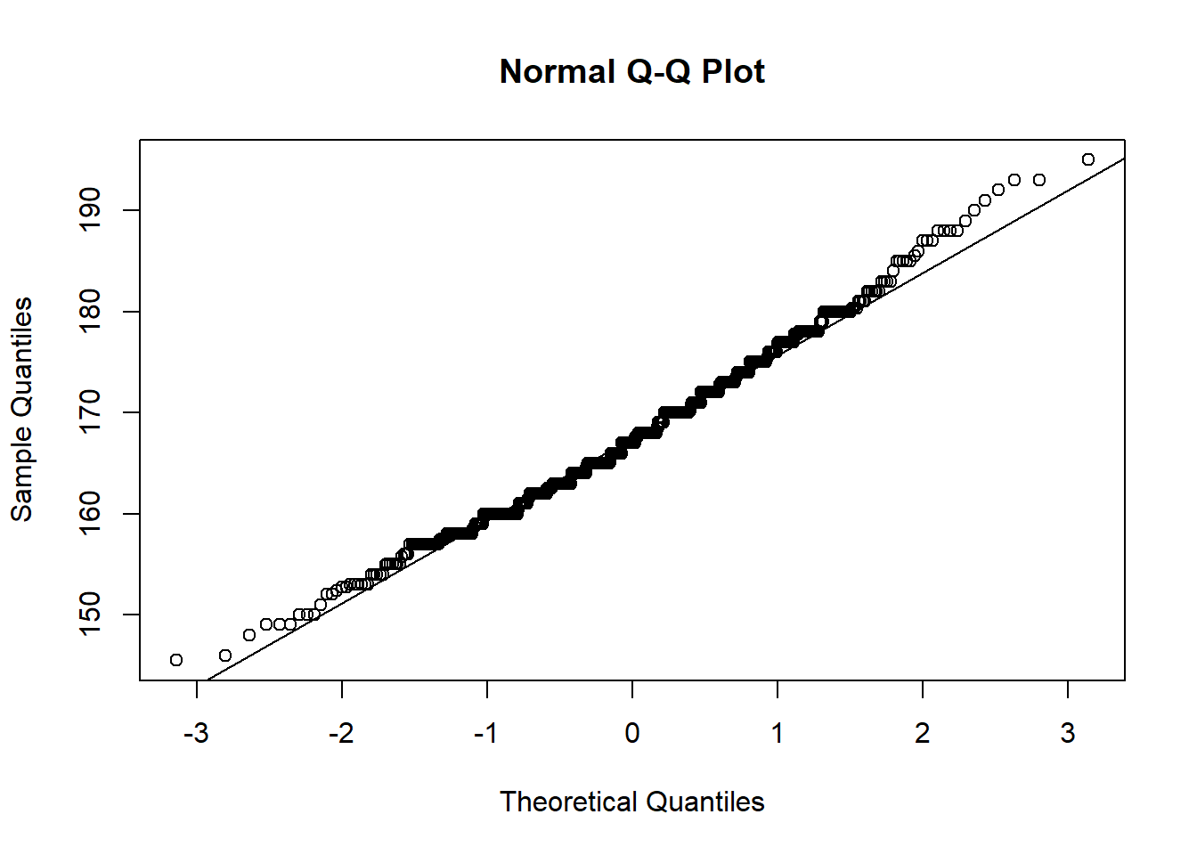
Make sure to consider the assumptions of the test!

Hints

• This is real data, and real data is rarely normal! If you conduct a Shapiro-Wilk test, you may well find \(p<.05\) and conclude that your data is not normal.
  So what do we do if a test indicates our assumptions are violated?
  Well, we should bear a couple of things in mind.
  1. A decision rule such as \(p<.05\) on Shapiro-Wilk test creates very dichotomous thinking for something which is in reality not black and white. Real life distributions are not either normal or non-normal. Plot the data, and make a judgement!
     
  2. As it happens, the t-test is actually reasonably robust against slight deviations from normality, especially if the sample size is “large enough” (rule-of-thumb n = 30) and the data are not heavily skewed. Plot your data and make a judgement!

Figure 2: The deeper you get into statistics, the more you discover that it is not simply a case of following step-by-step rules.

Solution 10.

Data

We’ll read in our data and check the dimensions and variable names

surveydata <- read_csv("https://uoepsy.github.io/data/usmr25survey_historical.csv")

dim(surveydata)

[1] 610  24

names(surveydata)

 [1] "birthmonth"        "height"            "eyecolour"        
 [4] "catdog"            "threewords"        "year"             
 [7] "course"            "in_uk"             "gender"           
[10] "optimism"          "spirituality"      "ampm"             
[13] "sleeprating"       "extraversion"      "agreeableness"    
[16] "conscientiousness" "emot_stability"    "imagination"      
[19] "loc"               "phone_unlocks"     "caffeine"         
[22] "caffeine_type"     "procrastination"   "multitasking"     

Descriptives

surveydata |> 
  summarise(
    mheight = mean(height, na.rm = T),
    sdheight = sd(height, na.rm = T),
    n = sum(!is.na(height))
  )

# A tibble: 1 × 3
  mheight sdheight     n
    <dbl>    <dbl> <int>
1    168.     8.41   597

Assumptions

The shapiro.test() suggests that our assumption of normality is not okay!
(the p-value is \(<.05\), suggesting that we reject the hypothesis that the data are drawn from a normally distributed population)

shapiro.test(surveydata$height)

    Shapiro-Wilk normality test

data:  surveydata$height
W = 0.99081, p-value = 0.0008986

However, as always, visualisations are vital here. The histogram below doesn’t look all that great, but the t.test is quite robust against slight violations of normality, especially as sample sizes increase beyond 30, and our data here actually looks fairly normal (this is a judgement call here - over time you will start to get a sense of what you might deem worrisome in these plots!).

ggplot(data = surveydata, aes(x = height)) + 
  geom_histogram(binwidth=2) +
  # adding our hypothesised mean
  geom_vline(xintercept = 165) 

We can also take a quick look at the QQplot. The points follow the line closely apart from at the tail ends, matching the heavier tails of the distribution that are visible in the histogram above.

qqnorm(surveydata$height)
qqline(surveydata$height)

The data are not very skewed, and together with the fact that we are working with a sample of 597, i feel fairly satisfied that the \(t\)-test will lead us to valid inferences.

t-test

t.test(surveydata$height, mu = 165, alternative = "two.sided")

    One Sample t-test

data:  surveydata$height
t = 7.832, df = 596, p-value = 2.209e-14
alternative hypothesis: true mean is not equal to 165
95 percent confidence interval:
 167.0192 168.3708
sample estimates:
mean of x 
  167.695 

Names and Tips

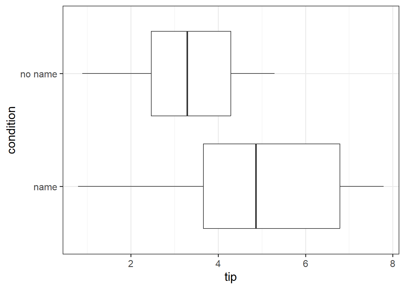
Research Question Can a server earn higher tips simply by introducing themselves by name when greeting customers?

Researchers investigated the effect of a server introducing herself by name on restaurant tipping. The study involved forty, 2-person parties eating a $23.21 fixed-price buffet Sunday brunch at Charley Brown’s Restaurant in Huntington Beach, California, on April 10 and 17, 1988.

Each two-person party was randomly assigned by the waitress to either a name or a no-name condition. The total amount paid by each party at the end of their meal was then recorded.

The data are available at https://uoepsy.github.io/data/gerritysim.csv
(This is a simulated example based on Garrity and Degelman (1990))

Question 11

Conduct an independent samples \(t\)-test to assess whether higher tips were earned when the server introduced themselves by name, in comparison to when they did not.

Hints

• There is a direction in the research question stated above, which means we will want to set alternative = ??.
  
• We’ll want to check the normality (either visually or with a test) of the variable of interest for each group.
  
• Some researchers suggest using the Welch t-test by default. This means you can relax the assumption of equal variances in the groups. If you want to test whether two variances are equal, try the var.test() function.

Solution 11.

Data

tipdata <- read_csv("https://uoepsy.github.io/data/gerritysim.csv")
dim(tipdata)

[1] 40  3

head(tipdata)

# A tibble: 6 × 3
   paid condition party
  <dbl> <chr>     <dbl>
1  28.5 name          1
2  27   no name       2
3  24.1 no name       3
4  28   name          4
5  30   name          5
6  27.5 name          6

It might be nice to conduct our analysis on just the tip given, and not the $23.21 meal price + tip.

#make a "tip" column, which is minus the meal amount
tipdata <- 
  tipdata |> mutate(
    tip = paid - 23.21
  )

Descriptives

tipdata |> 
  group_by(condition) |>
  summarise(
    meantip = mean(tip),
    sdtip = sd(tip)
  )

# A tibble: 2 × 3
  condition meantip sdtip
  <chr>       <dbl> <dbl>
1 name         4.94  1.88
2 no name      3.18  1.35

Plot

ggplot(data = tipdata, aes(x = tip, y = condition)) +
  geom_boxplot()

Assumptions

According to these tests, we have normally distributed data for both groups, with equal variances.

shapiro.test(tipdata$tip[tipdata$condition=="name"])

    Shapiro-Wilk normality test

data:  tipdata$tip[tipdata$condition == "name"]
W = 0.96267, p-value = 0.5985

shapiro.test(tipdata$tip[tipdata$condition=="no name"])

    Shapiro-Wilk normality test

data:  tipdata$tip[tipdata$condition == "no name"]
W = 0.94405, p-value = 0.2857

var.test(tip ~ condition, data = tipdata)

    F test to compare two variances

data:  tip by condition
F = 1.9344, num df = 19, denom df = 19, p-value = 0.1595
alternative hypothesis: true ratio of variances is not equal to 1
95 percent confidence interval:
 0.7656473 4.8870918
sample estimates:
ratio of variances 
           1.93437 

t-test

Because the variances do not appear to be unequal, we can actually use the standard t-test with var.equal = TRUE if we want. However, we’ll continue with the Welch t-test.

Remember that our alternative hypothesis here is that the average tips in the “name” condition is greater than in the “no name” condition.
R will take the levels in order here (alphabetically), and assume that the alternative is for that group, so we use alternative = "greater" here to say that the alternative is \(\text{name}-\text{no name} > 0\).

t.test(tip ~ condition, data = tipdata, alternative = "greater")

    Welch Two Sample t-test

data:  tip by condition
t = 3.4117, df = 34.502, p-value = 0.0008314
alternative hypothesis: true difference in means between group name and group no name is greater than 0
95 percent confidence interval:
 0.8893105       Inf
sample estimates:
   mean in group name mean in group no name 
               4.9450                3.1825 

Optional Extras

Here are a few extra questions for you to practice performing tests and making plots:

Optional Extra 1

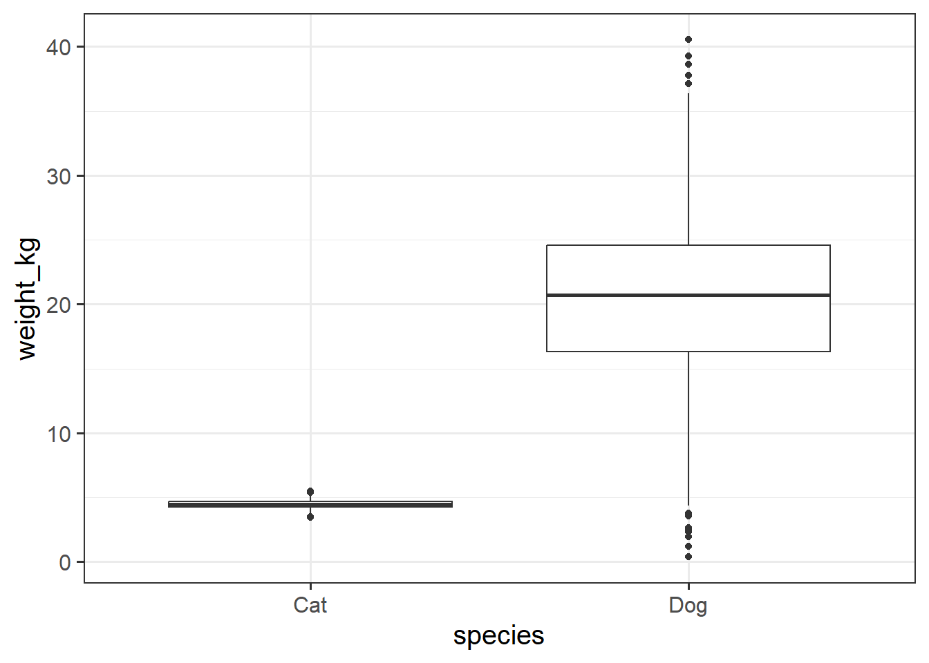
Are dogs heavier on average than cats?
Data from Week 1: https://uoepsy.github.io/data/pets_seattle.csv

Hints

• Remember from week 1 - not everything in that data is either a cat or a dog!

Solution 12.

pets <- read.csv("https://uoepsy.github.io/data/pets_seattle.csv")
catsndogs <- pets[pets$species != "Goat", ]

In this case, we want to test whether \(dogs > cats\). What we are testing then, whether \(dogs - cats > 0\) or \(cats - dogs < 0\).
By default, as the species variable is a character, it will use alphabetical ordering, and t.test() will test \(cats - dogs\). So we want our alternative hypothesis to be “less”:

t.test(weight_kg ~ species, catsndogs,
       alternative = "less")

An alternative is to set it as a factor, and specify the levels in the order we want:

catsndogs$species2 <- factor(catsndogs$species, levels = c("Dog","Cat"))

Which would then allow us to shove that into the t.test() and perform the same test, but using \(dogs - cats\) instead.

t.test(weight_kg ~ species2, catsndogs,
       alternative = "greater")

    Welch Two Sample t-test

data:  weight_kg by species2
t = 92.4, df = 1335.2, p-value < 2.2e-16
alternative hypothesis: true difference in means between group Dog and group Cat is greater than 0
95 percent confidence interval:
 15.60965      Inf
sample estimates:
mean in group Dog mean in group Cat 
        20.377489          4.484731 

catsndogs |>
  ggplot(aes(x=species,y=weight_kg)) + 
  geom_boxplot()

Optional Extra 2

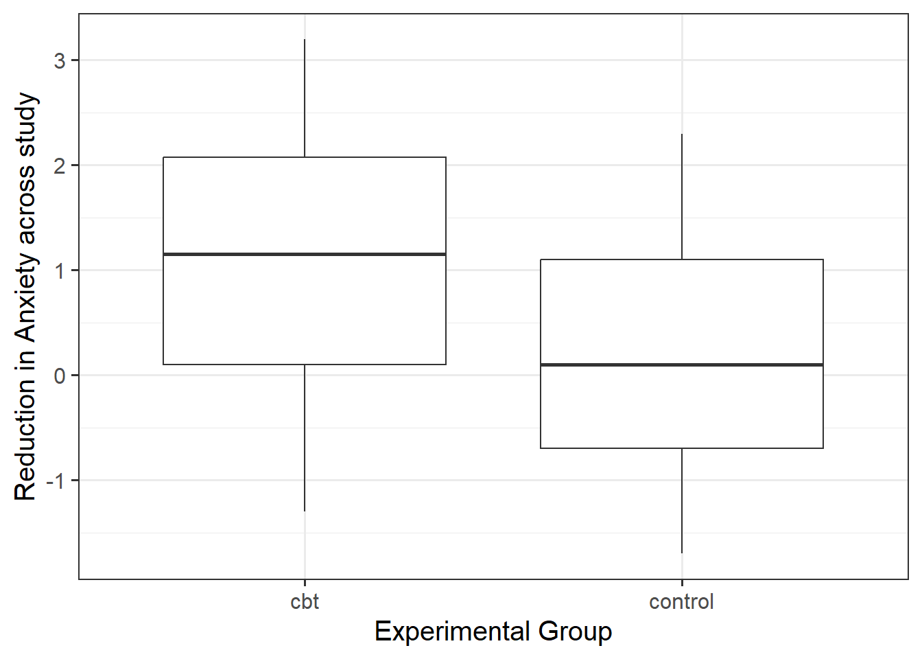
Is taking part in a cognitive behavioural therapy (CBT) based programme associated with a greater reduction, on average, in anxiety scores in comparison to a Control group?
Data are at https://uoepsy.github.io/data/cbtanx.csv . The dataset contains information on each person in an organisation, recording their professional role (management vs employee), whether they are allocated into the CBT programme or not (control vs cbt), and scores on anxiety at both the start and the end of the study period.

Hints

• you might have to make a new variable in order to test the research question.

Solution 13. Because we’re testing the reduction in anxiety, we need to calculate it. By subtracting anxiety at time 2 from anxiety at time 1, we create a variable for which bigger values represent more reduction in anxiety

cbtanx <- read.csv("https://uoepsy.github.io/data/cbtanx.csv")

cbtanx <- cbtanx |> mutate(reduction = anx_t1 - anx_t2)

And we can then test whether \(cbt - control > 0\):

t.test(reduction ~ cbt, data = cbtanx, 
       alternative = "greater")

    Welch Two Sample t-test

data:  reduction by cbt
t = 2.5953, df = 56.621, p-value = 0.006007
alternative hypothesis: true difference in means between group cbt and group control is greater than 0
95 percent confidence interval:
 0.2744051       Inf
sample estimates:
    mean in group cbt mean in group control 
            1.0266667             0.2551724 

And to make sure we’re getting things the right way around, make a plot:

ggplot(cbtanx, aes(x=cbt, y=reduction))+
  geom_boxplot() + 
  labs(x="Experimental Group",y="Reduction in Anxiety across study")

Optional Extra 3

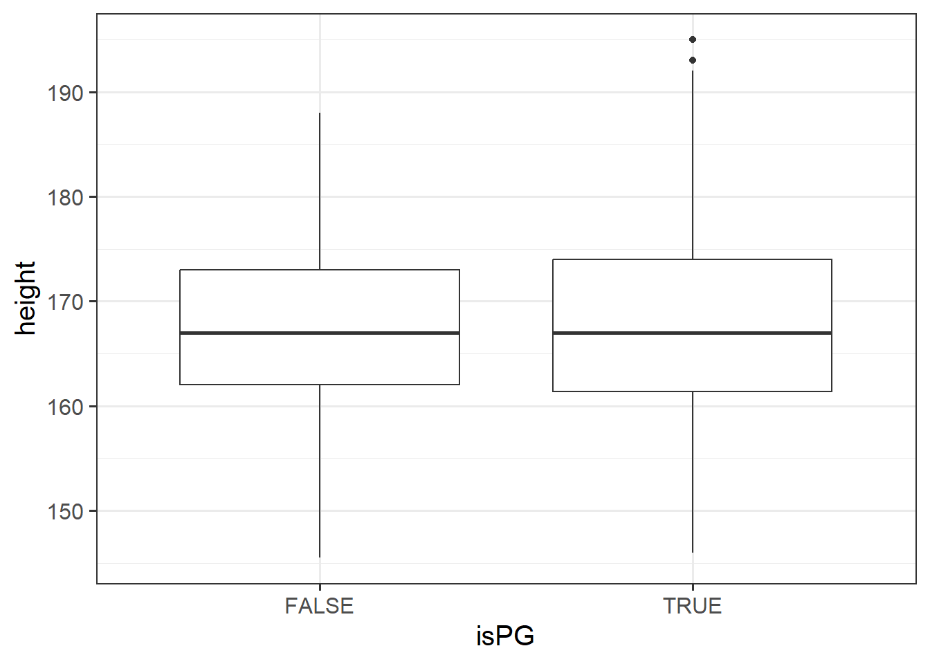
Are students on our postgraduate courses shorter/taller than those on our undergraduate courses?
We can again use the data from the past surveys: https://uoepsy.github.io/data/usmr25survey_historical.csv

“USMR” is our only postgraduate course.

Hints

• You’ll need to create a variable that identifies whether a respondent is from a postgrad or and undergrad course.

Solution 14.

surveydata <- read_csv("https://uoepsy.github.io/data/usmr25survey_historical.csv")
surveydata <- surveydata |>
  mutate(
    isPG = course=="usmr"
  )
table(surveydata$isPG)

FALSE  TRUE 
  240   370 

t.test(height ~ isPG, data = surveydata)

    Welch Two Sample t-test

data:  height by isPG
t = -0.22703, df = 547.46, p-value = 0.8205
alternative hypothesis: true difference in means between group FALSE and group TRUE is not equal to 0
95 percent confidence interval:
 -1.495371  1.185517
sample estimates:
mean in group FALSE  mean in group TRUE 
           167.6006            167.7555 

ggplot(surveydata, aes(x = isPG, y = height)) +
  geom_boxplot()

Footnotes

1. (Why 97.5? and not 95? We want the middle 95%, and \(t\)-distributions are symmetric, so we want to split that 5% in half, so that 2.5% is on either side. We could have also used qt(0.025, df = 6), which will just give us the same number but negative: -2.4469119)