Measurement Error and the need for SEM
We’ve been mentioning Structural Equation Modelling (SEM) for a few weeks now, but we haven’t been very clear on what exactly it is. Is it CFA? Is it Path Analysis? In fact it is both - it is the overarching framework of which CFA and Path Analysis are just parts.
The beauty comes in when we put these two approaches together.
Path analysis, as we saw last week, offers a way of specifying and evaluating a structural model, in which variables relate to one another in various ways, via different (sometimes indirect) paths. Common models like our old friend multiple regression can be expressed in a Path Analysis framework.
Factor Analysis, on the other hand, brings something absolutely crucial to the table - it allows us to mitigate some of the problems which are associated with measurement error by specifying the existence of some latent variable.
Combine them and we can reap the rewards of having both a structural model and a measurement model. The measurement model is our specification between the items we directly observed, and the latent variables of which we consider these items to be manifestations. The structural model is our specified model of the relationships between the latent variables.
Scale Scores
You will often find research that foregoes the measurement model by taking a scale score (i.e., the sum or mean of a set of likert-type questions).
This is what we did in the example in last week’s exercises, e.g.:
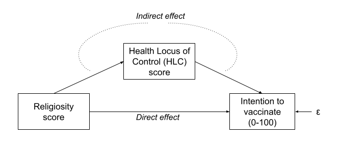
- Intention to vaccinate (scored on a range of 0-100.
- Health Locus of Control (HLC) score (average score on a set of items relating to perceived control over ones own health).
- Religiosity (average score on a set of items relating to an individual’s religiosity).
In doing so, we make the assumption that these variables provide measurements of the underlying latent construct without error. Furthermore, when taking the average score, we also make the assumption that each item is equally representative of our construct.
If you think about it, taking the mean of a set of items still has the sense of being a ‘factor structure’ in that we think of the items as being , but it constrains all our item variances to be equal, and all our factor loadings to be equal. So it doesn’t really have the benefits of a factor model.
Let’s demonstrate this, using a dataset from the CFA week exercises.
It doesn’t matter what it is for this example, so I’m just going to keep the first 4 items (it will save me typing out all the others!)
df <- read_csv("https://uoepsy.github.io/data/conduct_problems_2.csv")[,1:4]
head(df)
## # A tibble: 6 × 4
##    item1  item2   item3  item4
##    <dbl>  <dbl>   <dbl>  <dbl>
## 1 -0.968 -0.686 -0.342   0.600
## 2  0.275 -0.327 -0.0166 -1.08
## 3  0.255  0.826 -0.308  -1.15
## 4  1.73   1.67  -0.381   1.13
## 5 -0.464 -0.584 -0.507  -1.34
## 6 -0.501 -1.11  -0.310  -1.39
Now suppose that we are just going to take the mean of each persons score on the items, and use that as our measure of “conduct problems.”
We can achieve this easily with rowMeans()
# column bind the data with a column of the row means.
# only print the head of the data for now
cbind(df, mean = rowMeans(df)) %>% head
##    item1  item2   item3 item4   mean
## 1 -0.968 -0.686 -0.3418  0.60 -0.349
## 2  0.275 -0.327 -0.0166 -1.08 -0.286
## 3  0.255  0.826 -0.3077 -1.15 -0.094
## 4  1.725  1.667 -0.3810  1.13  1.034
## 5 -0.464 -0.584 -0.5072 -1.34 -0.724
## 6 -0.501 -1.108 -0.3097 -1.39 -0.826
Expressed as a factor model, what we are specifying is the below. Notice how we make it so that certain paths are identical by using a label i (for all factor loadings) and j (for all item variances).
mean_model <- '
    CP =~ i*item1 + i*item2 + i*item3 + i*item4
    item1 ~~ j*item1
    item2 ~~ j*item2
    item3 ~~ j*item3
    item4 ~~ j*item4
'
fitmean <- sem(mean_model, data = df)
We can obtain our factor scores using predict(). Let’s put them side-by-side with our rowMeans(), and we need to standardise them to get them in the same units:
factor_scores = scale(predict(fitmean))
rowmeans = scale(rowMeans(df))
cbind(factor_scores, rowmeans) %>% head
##           CP
## [1,] -0.3790 -0.3790
## [2,] -0.3035 -0.3035
## [3,] -0.0697 -0.0697
## [4,]  1.3001  1.3001
## [5,] -0.8343 -0.8343
## [6,] -0.9589 -0.9589
An alternative option would be to conduct a factor analysis where we allow our loadings to be estimated freely (without the equality constraint that is created by using a row-mean or a row-sum). We could then extract the factor scores, and then conduct a path analysis with those scores. This avoids the problem of equally weighting of items to construct, but does not solve our issue of the fact that these variables are imperfect measures of the latent construct.
Reliability
The accuracy and inconsistency with which an observed variable reflects the underlying construct that we consider it to be measuring is termed the reliability.
A silly example
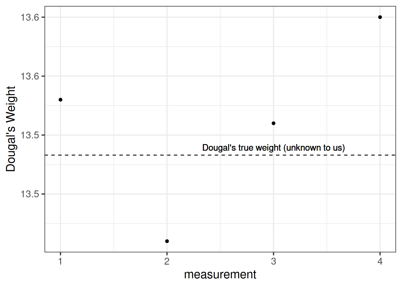
Suppose I’m trying to weigh my dog. I have a set of scales, and I put him on the scales. He weighs in at 13.53kg.
I immediately do it again, and the scales this time say 13.41kg. I do it again. 13.51kg, and again, 13.60kg.
What is happening? Is Dougal’s weight (Dougal is the dog, by the way) randomly fluctuating by 100g? Or are my scales just a bit inconsistent, and my observations contain measurement error?
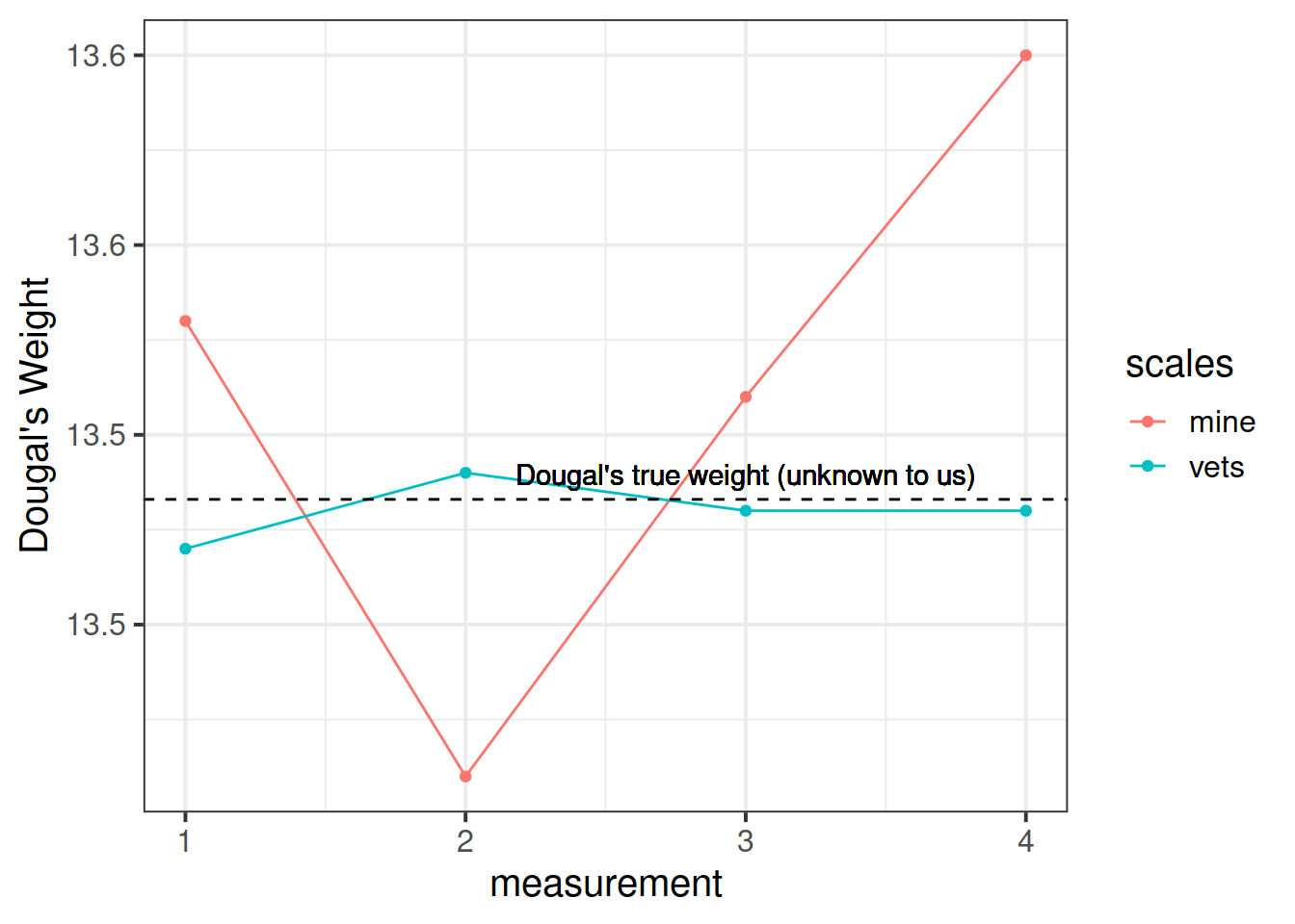
I take him to the vets, where they have a much better set of weighing scales, and I do the same thing (measure him 4 times). The weights are 13.47, 13.49, 13.48, 13.48.
The scales at the vets are clearly more reliable. We still don’t know Dougal’s true weight, but we are better informed to estimate it if we go on the measurements from the scales at the vet.
Another way to think about reliability is to take the view that \(\text{"observations = truth + error"}\), and more error = less reliable.
There are different types of reliability:
- test re-test reliability: correlation between values over repeated measurements.
- alternate-form reliability: correlation between scores on different forms/versions of a test (we might want different versions to avoid practice effects).
- Inter-rater reliability: correlation between values obtained from different raters.
The form of reliability we are going to be most concerned with here is known as Internal Consistency. This is the extent to which items within a scale are correlated with one another. There are two main measures of this:
alpha and omega
\[
\begin{align}
& \text{Cronbach's }\alpha = \frac{n \cdot \overline{cov(ij)}}{\overline{\sigma^2_i} + (n-1) \cdot \overline{cov(ij)}} & \\
& \text{Where:} \\
& n = \text{number of items} \\
& \overline{cov(ij)} = \text{average covariance between item-pairs} \\
& \overline{\sigma^2_i} = \text{average item variance} \\
\end{align}
\]
Ranges from 0 to 1 (higher is better).
You can get this using the alpha() function from the psych package. You just give it your items, and it will give you a value. In doing so, it just assumes that all items are of equal importance.
McDonald’s Omega \(\omega\) is substantially more complicated, but avoids the limitation that Cronbach’s alpha which assumes that all items are equally related to the construct. You can get it using the omega() function from the psych package. If you want more info about it then the help docs (?omega()) are a good place to start.
(Re)introducing SEM
After spending much of our time in the regression framework, the move to SEM can feel mind-boggling.
Give two researchers the same whiteboard on which your variables are drawn, and they may connect them in completely different ways. This flexibility can at first make SEM feel like a free-for-all (i.e., just do whatever you like, get a p-value out of it, and off we go!). However, to some people this is one of the main benefits: it forces you to be explicit in specifying your theory, and allows you to test your theory and examine how well it fits with the data you observed.
We have actually already go to grips with the starting point of how structural equation models work in the previous weeks.
- begin with an observed covariance matrix
- specify our our theoretical model
- fit our model to the data, with our estimation method (e.g. maximum likelihood) providing us with the set of parameter estimates for our model which best reproduce the observed covariance matrix.
- The estimated parameters for our model will not perfectly reproduce the covariance matrix, but they will give us a model implied covariance matrix. We can compare this to the observed covariance matrix in order to assess the fit of our theoretical model.
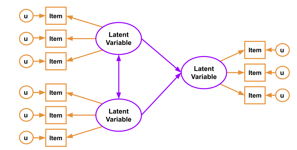
SEM allows us to account for measurement error by directly including it as part of the model - the residual variances of our indicator variables (the bits we have been labelling \(u\) our diagrams such as Figure 1) represent the measurement error (and other stray causes) associated with each observed variable.
If we had a latent variable which we considered to be measured without error by a number of items, then we would expect the covariances between the items measuring the latent variable to be exactly 1. However, we always have measurement error, meaning our correlations between items are attenuated (i.e, closer to zero). Modelling this attenuation of between-item correlations as error in measuring some underlying latent variable, allows us to estimate associations between latent variables (which aren’t directly measured, and so do not have measurement error associated with them).
Perhaps the easiest way to think of SEM is as a combination of the CFA approach (latent variables giving rise to our observed variables), and path analysis (where we test a model defined as a collection of paths between variables). In SEM we typically have two somewhat distinct parts: a measurement model (the CFA-like bits from latent variables to their indicators), and the structural model (the paths we are interested in, often between the latent variables). You can see an example below:
You can’t test the structural model if the measurement model is bad
If you test the relationships between a set of latent factors, and they are not reliably measured by the observed items, then this error propagates up to influence the fit of the structural model.
To test the measurement model, it is typical to saturate the structural model (i.e., allow all the latent variables to correlate with one another). This way any misfit is due to the measurement model only.
Fit Indices
Chi-Square - \(\chi^2\)
For structural equation models, a chi-square value can be obtained which reflects the discrepancy between the model-implied covariance matrix and the observed covariance matrix. We can then calculate a p-value for this chi-square statistic by using the chi-square distribution with the degrees of freedom equivalent to that of the model.
If we denote the population covariance matrix as \(\Sigma\) and the model-implied covariance matrix as \(\Sigma(\Theta)\), then we can think of the null hypothesis here as \(H_0: \Sigma - \Sigma(\Theta) = 0\). In this way our null hypothesis is that our theoretical model is correct (and can therefore perfectly reproduce the covariance matrix).
It is very sensitive to departures from normality, as well as sample size (for models with \(n>400\), the \(\chi^2\) is almost always significant), and can often lead to rejecting otherwise adequate models.
Absolute fit indices
“Absolute” measures of fit are based on comparing our model to a (hypothetical) perfectly fitted model. So we get an indication of “how far from perfect fit” our model is. Bigger values on these measures tend to indicate worse fit.
Standardised Root Mean Square Residual - SRMR
Standardised root mean square residual (SRMR) summarises the average covariance residuals (discrepancies between observed and model-implied covariance matrices). Smaller SRMR equates to better fit.
Common cut-offs for SRMR:
Root Mean Square Error of Approximation - RMSEA
The RMSEA is another measure of absolute fit, but it penalises for the complexity of the model. Based on the \(\chi^2/df\) ratio, this measure of fit is intended to take into account for the fact the model might hold approximately (rather than exactly) in the population.
Typical cut-offs for RMSEA:
- \(<0.05\) : Close fit
- \(>0.1\) : Poor fit
Incremental fit
“Incremental” fit indices are more similar to how we think about \(R^2\). A value of 0 is the worst possible fitting model, and values of 1 is the best possible fitting model. These fit indices compare the fit of the model to the that of a baseline model. In most cases, this is the null model, in which there are no relationships between latent variables (i.e., covariances among latent variables are all assumed to be zero).
Tucker Lewis Index (TLI) and Comparative Fit Index (CFI)
Both of these (TLI & CFI) are somewhat sensitive to the average size of correlations in the data. If the average correlation between variables is low, then these indices will not be very high.
Apparently (not sure where this comes from), TLI and CFI shouldn’t be considered if the RMSEA for the null model is \(<.158\) (you can quickly get the RMSEA for the null model by using nullRMSEA(my_fitted_model) from the semTools package).
Common cut-offs for TLI:
- \(<0.9\) : Poor fit
- \(1\) : Very good fit
- \(>1\) : Possible overfitting
Common cut-offs for CFI:
To compare multiple models
Akaike Information Criterion - AIC
Baysian Information Criterion - BIC
Sample Size Adjusted BIC - SSBIC
We have already been introduced to AIC and BIC in the regression world, but we now add to that the sample size adjusted BIC (SSBIC). These indices are only meaningful when making comparisons, meaning that two different models must be estimated. Lower values indicate better fit. comparing mode
The AIC is a comparative measure of fit and so it is meaningful only when two different models are estimated. Lower values indicate a better fit and so the model with the lowest AIC is the best fitting model. There are somewhat different formulas given for the AIC in the literature, but those differences are not really meaningful as it is the difference in AIC that really matters:
Local Fit (Modification Indices)
In addition to the overall fit of our model, we can look at specific parameters, the inclusion of which may improve model fit. These are known as modification indices, and you can get them from passing a SEM object to modindices() or modificationindices(). They provide the estimated value for each additional parameter, and the improvement in the \(\chi^2\) value that would be obtained with its addition to the model. Note that it will be tempting to look at modification indices and start adding to your model to improve fit, but this should be strongly guided by whether the additional paths make theoretical sense. Additionally, once a path is added, and modification indices are computed on the new model, you may find some completely different paths are suggested as possibly modification indices!
Exercises
A researcher wants to apply the theory of planned behaviour to understand engagement in physical activity. The theory of planned behaviour is summarised in Figure 2 (only the latent variables and not the items are shown). Attitudes refer to the extent to which a person had a favourable view of exercising; subjective norms refer to whether they believe others whose opinions they care about believe exercise to be a good thing; and perceived behavioural control refers to the extent to which they believe exercising is under their control. Intentions refer to whether a person intends to exercise and ‘behaviour’ is a measure of the extent to which they exercised. Each construct is measured using four items.
The data is available either:
Question A1
Did you do the final exercise (writing up your results) from last week? Our example write-up is now visible (see last week) against which you can compare yours.
Please note: Writing-up is an important skill, and attempting these questions yourself (rather than simply reading through the example write-ups) will help a lot when it comes to writing your assessment.
Question A2
Read in the data using the appropriate function. We’ve given you .csv files for a long time now, but it’s good to be prepared to encounter all sorts of weird filetypes.
Can you successfully read in from both types of data?
Solution
Either one or the other of:
load(url("https://uoepsy.github.io/data/TPB_data.Rdata"))

TPB_data <- read.table("https://uoepsy.github.io/data/TPB_data.txt", header = TRUE, sep = "\t")
Question A3
Test separate one-factor models for each construct.
Are the measurement models satisfactory? (check their fit measures).
Solution
# specify one factor CFA model for attitudes
attitude_model <- 'att =~ attitude1 + attitude2 + attitude3 + attitude4'
# estimate the model
attitude_model.est <- cfa(attitude_model, data=TPB_data)
# inspect the output
summary(attitude_model.est, fit.measures=T, standardized=T)
## lavaan 0.6-8 ended normally after 19 iterations
##
##   Estimator                                         ML
##   Optimization method                           NLMINB
##   Number of model parameters                         8
##
##   Number of observations                           890
##
## Model Test User Model:
##
##   Test statistic                                 0.175
##   Degrees of freedom                                 2
##   P-value (Chi-square)                           0.916
##
## Model Test Baseline Model:
##
##   Test statistic                              1032.173
##   Degrees of freedom                                 6
##   P-value                                        0.000
##
## User Model versus Baseline Model:
##
##   Comparative Fit Index (CFI)                    1.000
##   Tucker-Lewis Index (TLI)                       1.005
##
## Loglikelihood and Information Criteria:
##
##   Loglikelihood user model (H0)              -4620.704
##   Loglikelihood unrestricted model (H1)      -4620.616
##
##   Akaike (AIC)                                9257.408
##   Bayesian (BIC)                              9295.737
##   Sample-size adjusted Bayesian (BIC)         9270.331
##
## Root Mean Square Error of Approximation:
##
##   RMSEA                                          0.000
##   90 Percent confidence interval - lower         0.000
##   90 Percent confidence interval - upper         0.025
##   P-value RMSEA <= 0.05                          0.990
##
## Standardized Root Mean Square Residual:
##
##   SRMR                                           0.002
##
## Parameter Estimates:
##
##   Standard errors                             Standard
##   Information                                 Expected
##   Information saturated (h1) model          Structured
##
## Latent Variables:
##                    Estimate  Std.Err  z-value  P(>|z|)   Std.lv  Std.all
##   att =~
##     attitude1         1.000                               0.705    0.685
##     attitude2         1.052    0.062   17.093    0.000    0.742    0.722
##     attitude3         0.989    0.060   16.432    0.000    0.698    0.681
##     attitude4         1.060    0.061   17.270    0.000    0.747    0.736
##
## Variances:
##                    Estimate  Std.Err  z-value  P(>|z|)   Std.lv  Std.all
##    .attitude1         0.562    0.035   16.245    0.000    0.562    0.531
##    .attitude2         0.505    0.033   15.077    0.000    0.505    0.478
##    .attitude3         0.563    0.034   16.365    0.000    0.563    0.537
##    .attitude4         0.474    0.032   14.582    0.000    0.474    0.459
##     att               0.497    0.048   10.371    0.000    1.000    1.000
#check the model fit and that RMSEA<.05, SRMR<.05, TLI>0.95 and CFI>.95 and that all loadings are significant and >|.30|
modificationindices(attitude_model.est)
##          lhs op       rhs    mi    epc sepc.lv sepc.all sepc.nox
## 10 attitude1 ~~ attitude2 0.040 -0.006  -0.006   -0.011   -0.011
## 11 attitude1 ~~ attitude3 0.049 -0.006  -0.006   -0.011   -0.011
## 12 attitude1 ~~ attitude4 0.176  0.013   0.013    0.025    0.025
## 13 attitude2 ~~ attitude3 0.176  0.013   0.013    0.024    0.024
## 14 attitude2 ~~ attitude4 0.049 -0.007  -0.007   -0.015   -0.015
## 15 attitude3 ~~ attitude4 0.040 -0.006  -0.006   -0.012   -0.012
#check the largest modification indices to see if the expected parameter changes are large enough to justify any additional parameters in the model
The above code shows you the steps you should run through for the attitudes construct. You should repeat these steps for each of:
- attitudes
- subjective norms
- perceived behavioural control
- intentions
- behaviour
Question A4
Using lavaan syntax, specify a structural equation model that corresponds to the model in Figure 2. For each construct use a latent variable measured by the corresponding items in the dataset.
Solution
TPB_model<-'
#measurement models for attitudes, subjective norms and perceived behavioural control

  att =~ attitude1 + attitude2 + attitude3 + attitude4
  SN =~ SN1 + SN2 + SN3 + SN4
  PBC =~ PBC1 + PBC2 + PBC3 + PBC4
  intent =~ int1 + int2 + int3 + int4
  beh =~ beh1 + beh2 + beh3 + beh4

#regressions

  beh ~ intent + PBC
  intent ~ att + SN + PBC

#covariances between attitudes, subjective norms and perceived behavioural control

  att ~~ SN
  att ~~ PBC
  SN ~~ PBC
'
Question A5
Estimate the model from Question A4 and evaluate the model
- Does the model fit well?
- Are the hypothesised paths significant?
Solution
We can estimate the model using the sem() function.
By default the sem() function will scale the latent variables by fixing the loading of the first item for each latent variable to 1 but we can override this by setting std.lv=T if we wanted to. By default, maximum likelihood estimation will be used.
TPB_model.est<-sem(TPB_model, data=TPB_data, std.lv=T)

summary(TPB_model.est, fit.measures=T, standardized=T)
## lavaan 0.6-8 ended normally after 24 iterations
##
##   Estimator                                         ML
##   Optimization method                           NLMINB
##   Number of model parameters                        48
##
##   Number of observations                           890
##
## Model Test User Model:
##
##   Test statistic                               157.059
##   Degrees of freedom                               162
##   P-value (Chi-square)                           0.595
##
## Model Test Baseline Model:
##
##   Test statistic                              5335.624
##   Degrees of freedom                               190
##   P-value                                        0.000
##
## User Model versus Baseline Model:
##
##   Comparative Fit Index (CFI)                    1.000
##   Tucker-Lewis Index (TLI)                       1.001
##
## Loglikelihood and Information Criteria:
##
##   Loglikelihood user model (H0)             -24403.833
##   Loglikelihood unrestricted model (H1)     -24325.304
##
##   Akaike (AIC)                               48903.667
##   Bayesian (BIC)                             49133.646
##   Sample-size adjusted Bayesian (BIC)        48981.207
##
## Root Mean Square Error of Approximation:
##
##   RMSEA                                          0.000
##   90 Percent confidence interval - lower         0.000
##   90 Percent confidence interval - upper         0.014
##   P-value RMSEA <= 0.05                          1.000
##
## Standardized Root Mean Square Residual:
##
##   SRMR                                           0.023
##
## Parameter Estimates:
##
##   Standard errors                             Standard
##   Information                                 Expected
##   Information saturated (h1) model          Structured
##
## Latent Variables:
##                    Estimate  Std.Err  z-value  P(>|z|)   Std.lv  Std.all
##   att =~
##     attitude1         0.710    0.034   21.152    0.000    0.710    0.689
##     attitude2         0.746    0.033   22.590    0.000    0.746    0.726
##     attitude3         0.707    0.033   21.155    0.000    0.707    0.689
##     attitude4         0.730    0.033   22.298    0.000    0.730    0.719
##   SN =~
##     SN1               0.685    0.036   18.786    0.000    0.685    0.661
##     SN2               0.673    0.036   18.466    0.000    0.673    0.651
##     SN3               0.646    0.037   17.369    0.000    0.646    0.616
##     SN4               0.681    0.038   18.064    0.000    0.681    0.638
##   PBC =~
##     PBC1              0.776    0.029   27.045    0.000    0.776    0.799
##     PBC2              0.728    0.028   25.777    0.000    0.728    0.772
##     PBC3              0.709    0.028   25.023    0.000    0.709    0.756
##     PBC4              0.747    0.029   25.813    0.000    0.747    0.773
##   intent =~
##     int1              0.459    0.033   14.067    0.000    0.708    0.584
##     int2              0.535    0.035   15.144    0.000    0.824    0.646
##     int3              0.513    0.035   14.794    0.000    0.791    0.625
##     int4              0.492    0.034   14.300    0.000    0.759    0.597
##   beh =~
##     beh1              0.623    0.039   16.044    0.000    0.808    0.649
##     beh2              0.584    0.039   15.022    0.000    0.758    0.599
##     beh3              0.576    0.039   14.782    0.000    0.748    0.588
##     beh4              0.599    0.040   15.153    0.000    0.777    0.605
##
## Regressions:
##                    Estimate  Std.Err  z-value  P(>|z|)   Std.lv  Std.all
##   beh ~
##     intent            0.426    0.057    7.513    0.000    0.506    0.506
##     PBC               0.241    0.071    3.373    0.001    0.185    0.185
##   intent ~
##     att               0.553    0.069    8.010    0.000    0.359    0.359
##     SN                0.302    0.064    4.692    0.000    0.196    0.196
##     PBC               0.756    0.073   10.364    0.000    0.490    0.490
##
## Covariances:
##                    Estimate  Std.Err  z-value  P(>|z|)   Std.lv  Std.all
##   att ~~
##     SN                0.320    0.040    7.938    0.000    0.320    0.320
##     PBC               0.253    0.038    6.611    0.000    0.253    0.253
##   SN ~~
##     PBC               0.196    0.041    4.800    0.000    0.196    0.196
##
## Variances:
##                    Estimate  Std.Err  z-value  P(>|z|)   Std.lv  Std.all
##    .attitude1         0.556    0.034   16.511    0.000    0.556    0.525
##    .attitude2         0.498    0.032   15.415    0.000    0.498    0.472
##    .attitude3         0.551    0.033   16.509    0.000    0.551    0.525
##    .attitude4         0.498    0.032   15.658    0.000    0.498    0.483
##    .SN1               0.605    0.039   15.384    0.000    0.605    0.563
##    .SN2               0.616    0.039   15.689    0.000    0.616    0.577
##    .SN3               0.681    0.041   16.608    0.000    0.681    0.620
##    .SN4               0.676    0.042   16.047    0.000    0.676    0.593
##    .PBC1              0.341    0.023   15.163    0.000    0.341    0.362
##    .PBC2              0.359    0.022   16.144    0.000    0.359    0.404
##    .PBC3              0.377    0.023   16.639    0.000    0.377    0.429
##    .PBC4              0.376    0.023   16.119    0.000    0.376    0.403
##    .int1              0.969    0.054   18.096    0.000    0.969    0.659
##    .int2              0.949    0.056   16.914    0.000    0.949    0.583
##    .int3              0.976    0.056   17.371    0.000    0.976    0.610
##    .int4              1.042    0.058   17.889    0.000    1.042    0.644
##    .beh1              0.900    0.057   15.656    0.000    0.900    0.579
##    .beh2              1.026    0.061   16.918    0.000    1.026    0.641
##    .beh3              1.057    0.062   17.152    0.000    1.057    0.654
##    .beh4              1.045    0.062   16.783    0.000    1.045    0.634
##     att               1.000                               1.000    1.000
##     SN                1.000                               1.000    1.000
##     PBC               1.000                               1.000    1.000
##    .intent            1.000                               0.421    0.421
##    .beh               1.000                               0.593    0.593
We can see that the model fits well according to RMSEA, SRMR, TLI and CFI. All of the hypothesised paths in the theory of planned behaviour are statistically significant.
Question A6
Examine the modification indices and expected parameter changes - are there any additional parameters you would consider including?
Solution
modindices(TPB_model.est)
##           lhs op       rhs     mi    epc sepc.lv sepc.all sepc.nox
## 54        att =~       SN1  1.663  0.049   0.049    0.047    0.047
## 55        att =~       SN2  3.197  0.067   0.067    0.065    0.065
## 56        att =~       SN3  1.283 -0.043  -0.043   -0.041   -0.041
## 57        att =~       SN4  4.294 -0.081  -0.081   -0.076   -0.076
## 58        att =~      PBC1  0.350 -0.016  -0.016   -0.017   -0.017
## 59        att =~      PBC2  1.394  0.032   0.032    0.034    0.034
## 60        att =~      PBC3  0.133 -0.010  -0.010   -0.011   -0.011
## 61        att =~      PBC4  0.043 -0.006  -0.006   -0.006   -0.006
## 62        att =~      int1  0.002 -0.003  -0.003   -0.002   -0.002
## 63        att =~      int2  0.014 -0.007  -0.007   -0.005   -0.005
## 64        att =~      int3  0.379  0.035   0.035    0.027    0.027
## 65        att =~      int4  0.243 -0.028  -0.028   -0.022   -0.022
## 66        att =~      beh1  0.134 -0.016  -0.016   -0.013   -0.013
## 67        att =~      beh2  0.844  0.042   0.042    0.034    0.034
## 68        att =~      beh3  0.033  0.008   0.008    0.007    0.007
## 69        att =~      beh4  0.420 -0.030  -0.030   -0.024   -0.024
## 70         SN =~ attitude1  0.923  0.035   0.035    0.034    0.034
## 71         SN =~ attitude2  0.454  0.024   0.024    0.023    0.023
## 72         SN =~ attitude3  0.054  0.008   0.008    0.008    0.008
## 73         SN =~ attitude4  3.291 -0.064  -0.064   -0.063   -0.063
## 74         SN =~      PBC1  0.216 -0.013  -0.013   -0.013   -0.013
## 75         SN =~      PBC2  1.679  0.036   0.036    0.038    0.038
## 76         SN =~      PBC3  0.485 -0.019  -0.019   -0.021   -0.021
## 77         SN =~      PBC4  0.034 -0.005  -0.005   -0.005   -0.005
## 78         SN =~      int1  2.659 -0.080  -0.080   -0.066   -0.066
## 79         SN =~      int2  0.050 -0.011  -0.011   -0.009   -0.009
## 80         SN =~      int3  0.269  0.027   0.027    0.021    0.021
## 81         SN =~      int4  1.081  0.054   0.054    0.042    0.042
## 82         SN =~      beh1  2.904 -0.075  -0.075   -0.060   -0.060
## 83         SN =~      beh2  0.263  0.023   0.023    0.019    0.019
## 84         SN =~      beh3  1.906  0.064   0.064    0.050    0.050
## 85         SN =~      beh4  0.202  0.021   0.021    0.016    0.016
## 86        PBC =~ attitude1  1.435 -0.039  -0.039   -0.038   -0.038
## 87        PBC =~ attitude2  0.256  0.016   0.016    0.016    0.016
## 88        PBC =~ attitude3  1.785  0.043   0.043    0.042    0.042
## 89        PBC =~ attitude4  0.415 -0.020  -0.020   -0.020   -0.020
## 90        PBC =~       SN1  0.103  0.011   0.011    0.011    0.011
## 91        PBC =~       SN2  1.946  0.048   0.048    0.046    0.046
## 92        PBC =~       SN3  3.081 -0.061  -0.061   -0.058   -0.058
## 93        PBC =~       SN4  0.005 -0.002  -0.002   -0.002   -0.002
## 94        PBC =~      int1  0.043 -0.012  -0.012   -0.010   -0.010
## 95        PBC =~      int2  0.064  0.016   0.016    0.012    0.012
## 96        PBC =~      int3  0.000  0.001   0.001    0.001    0.001
## 97        PBC =~      int4  0.007 -0.005  -0.005   -0.004   -0.004
## 98        PBC =~      beh1  0.005 -0.004  -0.004   -0.003   -0.003
## 99        PBC =~      beh2  1.367  0.063   0.063    0.050    0.050
## 100       PBC =~      beh3  0.001 -0.001  -0.001   -0.001   -0.001
## 101       PBC =~      beh4  1.119 -0.058  -0.058   -0.045   -0.045
## 102    intent =~ attitude1  0.043  0.006   0.009    0.009    0.009
## 103    intent =~ attitude2  0.353  0.016   0.025    0.025    0.025
## 104    intent =~ attitude3  3.425  0.051   0.079    0.077    0.077
## 105    intent =~ attitude4  6.558 -0.070  -0.108   -0.106   -0.106
## 106    intent =~       SN1  0.024  0.004   0.006    0.006    0.006
## 107    intent =~       SN2  4.489  0.056   0.086    0.084    0.084
## 108    intent =~       SN3  1.063 -0.028  -0.043   -0.041   -0.041
## 109    intent =~       SN4  1.761 -0.036  -0.056   -0.052   -0.052
## 110    intent =~      PBC1  0.058 -0.006  -0.009   -0.010   -0.010
## 111    intent =~      PBC2  0.656  0.020   0.031    0.033    0.033
## 112    intent =~      PBC3  0.069 -0.007  -0.010   -0.011   -0.011
## 113    intent =~      PBC4  0.092 -0.008  -0.012   -0.012   -0.012
## 114    intent =~      beh1  0.008  0.004   0.006    0.005    0.005
## 115    intent =~      beh2  0.306 -0.025  -0.039   -0.031   -0.031
## 116    intent =~      beh3  1.632  0.059   0.091    0.071    0.071
## 117    intent =~      beh4  0.630 -0.037  -0.057   -0.044   -0.044
## 118       beh =~ attitude1  0.187 -0.012  -0.016   -0.015   -0.015
## 119       beh =~ attitude2  1.049 -0.028  -0.036   -0.035   -0.035
## 120       beh =~ attitude3  6.156  0.068   0.089    0.087    0.087
## 121       beh =~ attitude4  0.815 -0.024  -0.031   -0.031   -0.031
## 122       beh =~       SN1  0.084  0.008   0.011    0.010    0.010
## 123       beh =~       SN2  1.865  0.039   0.051    0.049    0.049
## 124       beh =~       SN3  2.447 -0.046  -0.059   -0.057   -0.057
## 125       beh =~       SN4  0.009  0.003   0.004    0.003    0.003
## 126       beh =~      PBC1  0.923  0.026   0.033    0.034    0.034
## 127       beh =~      PBC2  0.127 -0.009  -0.012   -0.013   -0.013
## 128       beh =~      PBC3  0.478  0.018   0.024    0.025    0.025
## 129       beh =~      PBC4  1.692 -0.035  -0.046   -0.047   -0.047
## 130       beh =~      int1  0.556 -0.038  -0.049   -0.040   -0.040
## 131       beh =~      int2  1.705  0.069   0.089    0.070    0.070
## 132       beh =~      int3  0.140 -0.020  -0.025   -0.020   -0.020
## 133       beh =~      int4  0.260 -0.027  -0.035   -0.027   -0.027
## 134 attitude1 ~~ attitude2  0.587 -0.022  -0.022   -0.041   -0.041
## 135 attitude1 ~~ attitude3  0.930 -0.026  -0.026   -0.048   -0.048
## 136 attitude1 ~~ attitude4  1.278  0.031   0.031    0.059    0.059
## 137 attitude1 ~~       SN1  0.738  0.021   0.021    0.035    0.035
## 138 attitude1 ~~       SN2  0.068  0.006   0.006    0.011    0.011
## 139 attitude1 ~~       SN3  0.258  0.013   0.013    0.020    0.020
## 140 attitude1 ~~       SN4  0.446 -0.017  -0.017   -0.027   -0.027
## 141 attitude1 ~~      PBC1  2.436 -0.029  -0.029   -0.066   -0.066
## 142 attitude1 ~~      PBC2  0.070 -0.005  -0.005   -0.011   -0.011
## 143 attitude1 ~~      PBC3  0.033  0.003   0.003    0.007    0.007
## 144 attitude1 ~~      PBC4  0.031  0.003   0.003    0.007    0.007
## 145 attitude1 ~~      int1  0.075  0.008   0.008    0.011    0.011
## 146 attitude1 ~~      int2  0.476 -0.020  -0.020   -0.028   -0.028
## 147 attitude1 ~~      int3  3.310  0.054   0.054    0.073    0.073
## 148 attitude1 ~~      int4  0.254  0.015   0.015    0.020    0.020
## 149 attitude1 ~~      beh1  1.811  0.039   0.039    0.055    0.055
## 150 attitude1 ~~      beh2  0.045  0.006   0.006    0.008    0.008
## 151 attitude1 ~~      beh3  0.490 -0.021  -0.021   -0.028   -0.028
## 152 attitude1 ~~      beh4  2.283 -0.046  -0.046   -0.060   -0.060
## 153 attitude2 ~~ attitude3  0.234 -0.014  -0.014   -0.026   -0.026
## 154 attitude2 ~~ attitude4  0.582  0.022   0.022    0.044    0.044
## 155 attitude2 ~~       SN1  9.972  0.073   0.073    0.133    0.133
## 156 attitude2 ~~       SN2  2.493 -0.037  -0.037   -0.066   -0.066
## 157 attitude2 ~~       SN3  0.257 -0.012  -0.012   -0.021   -0.021
## 158 attitude2 ~~       SN4  0.314 -0.014  -0.014   -0.023   -0.023
## 159 attitude2 ~~      PBC1  0.342 -0.010  -0.010   -0.025   -0.025
## 160 attitude2 ~~      PBC2  0.529  0.013   0.013    0.031    0.031
## 161 attitude2 ~~      PBC3  0.302  0.010   0.010    0.023    0.023
## 162 attitude2 ~~      PBC4  0.002 -0.001  -0.001   -0.002   -0.002
## 163 attitude2 ~~      int1  2.209  0.042   0.042    0.060    0.060
## 164 attitude2 ~~      int2  0.020 -0.004  -0.004   -0.006   -0.006
## 165 attitude2 ~~      int3  0.001 -0.001  -0.001   -0.001   -0.001
## 166 attitude2 ~~      int4  0.063  0.007   0.007    0.010    0.010
## 167 attitude2 ~~      beh1  0.447 -0.019  -0.019   -0.028   -0.028
## 168 attitude2 ~~      beh2  1.233  0.032   0.032    0.045    0.045
## 169 attitude2 ~~      beh3  8.914 -0.088  -0.088   -0.121   -0.121
## 170 attitude2 ~~      beh4  0.000  0.000   0.000    0.000    0.000
## 171 attitude3 ~~ attitude4  0.084  0.008   0.008    0.015    0.015
## 172 attitude3 ~~       SN1  2.870 -0.040  -0.040   -0.070   -0.070
## 173 attitude3 ~~       SN2  4.497  0.051   0.051    0.087    0.087
## 174 attitude3 ~~       SN3  0.029 -0.004  -0.004   -0.007   -0.007
## 175 attitude3 ~~       SN4  0.303 -0.014  -0.014   -0.022   -0.022
## 176 attitude3 ~~      PBC1  1.372  0.021   0.021    0.049    0.049
## 177 attitude3 ~~      PBC2  0.044  0.004   0.004    0.009    0.009
## 178 attitude3 ~~      PBC3  0.001  0.000   0.000   -0.001   -0.001
## 179 attitude3 ~~      PBC4  1.608 -0.024  -0.024   -0.052   -0.052
## 180 attitude3 ~~      int1  0.005  0.002   0.002    0.003    0.003
## 181 attitude3 ~~      int2  0.112  0.010   0.010    0.014    0.014
## 182 attitude3 ~~      int3  0.005  0.002   0.002    0.003    0.003
## 183 attitude3 ~~      int4  0.031  0.005   0.005    0.007    0.007
## 184 attitude3 ~~      beh1  0.123 -0.010  -0.010   -0.014   -0.014
## 185 attitude3 ~~      beh2  0.000  0.000   0.000    0.000    0.000
## 186 attitude3 ~~      beh3  3.529  0.057   0.057    0.074    0.074
## 187 attitude3 ~~      beh4  1.412  0.036   0.036    0.047    0.047
## 188 attitude4 ~~       SN1  0.783 -0.020  -0.020   -0.037   -0.037
## 189 attitude4 ~~       SN2  0.173  0.010   0.010    0.017    0.017
## 190 attitude4 ~~       SN3  0.696 -0.020  -0.020   -0.034   -0.034
## 191 attitude4 ~~       SN4  0.000  0.000   0.000    0.001    0.001
## 192 attitude4 ~~      PBC1  0.143  0.007   0.007    0.016    0.016
## 193 attitude4 ~~      PBC2  0.063  0.004   0.004    0.011    0.011
## 194 attitude4 ~~      PBC3  0.901 -0.017  -0.017   -0.039   -0.039
## 195 attitude4 ~~      PBC4  0.964  0.018   0.018    0.041    0.041
## 196 attitude4 ~~      int1  2.923 -0.048  -0.048   -0.069   -0.069
## 197 attitude4 ~~      int2  0.170  0.012   0.012    0.017    0.017
## 198 attitude4 ~~      int3  1.396 -0.034  -0.034   -0.048   -0.048
## 199 attitude4 ~~      int4  2.376 -0.045  -0.045   -0.062   -0.062
## 200 attitude4 ~~      beh1  0.276 -0.015  -0.015   -0.022   -0.022
## 201 attitude4 ~~      beh2  0.036  0.006   0.006    0.008    0.008
## 202 attitude4 ~~      beh3  1.806  0.039   0.039    0.054    0.054
## 203 attitude4 ~~      beh4  0.122 -0.010  -0.010   -0.014   -0.014
## 204       SN1 ~~       SN2  3.906 -0.069  -0.069   -0.114   -0.114
## 205       SN1 ~~       SN3  1.516  0.042   0.042    0.066    0.066
## 206       SN1 ~~       SN4  0.187  0.015   0.015    0.024    0.024
## 207       SN1 ~~      PBC1  0.563 -0.015  -0.015   -0.032   -0.032
## 208       SN1 ~~      PBC2  0.396  0.012   0.012    0.026    0.026
## 209       SN1 ~~      PBC3  1.548  0.025   0.025    0.051    0.051
## 210       SN1 ~~      PBC4  0.348 -0.012  -0.012   -0.025   -0.025
## 211       SN1 ~~      int1  0.183 -0.013  -0.013   -0.017   -0.017
## 212       SN1 ~~      int2  0.117 -0.011  -0.011   -0.014   -0.014
## 213       SN1 ~~      int3  2.133 -0.045  -0.045   -0.059   -0.059
## 214       SN1 ~~      int4  0.802  0.028   0.028    0.036    0.036
## 215       SN1 ~~      beh1  0.345  0.018   0.018    0.024    0.024
## 216       SN1 ~~      beh2  0.044 -0.007  -0.007   -0.008   -0.008
## 217       SN1 ~~      beh3  3.760 -0.062  -0.062   -0.078   -0.078
## 218       SN1 ~~      beh4  2.978  0.056   0.056    0.070    0.070
## 219       SN2 ~~       SN3  0.193 -0.015  -0.015   -0.023   -0.023
## 220       SN2 ~~       SN4  0.946  0.034   0.034    0.053    0.053
## 221       SN2 ~~      PBC1  0.086  0.006   0.006    0.012    0.012
## 222       SN2 ~~      PBC2  0.099  0.006   0.006    0.013    0.013
## 223       SN2 ~~      PBC3  0.271 -0.010  -0.010   -0.021   -0.021
## 224       SN2 ~~      PBC4  0.077  0.006   0.006    0.012    0.012
## 225       SN2 ~~      int1  0.014 -0.004  -0.004   -0.005   -0.005
## 226       SN2 ~~      int2  1.097  0.033   0.033    0.043    0.043
## 227       SN2 ~~      int3  0.058 -0.008  -0.008   -0.010   -0.010
## 228       SN2 ~~      int4  0.343  0.019   0.019    0.023    0.023
## 229       SN2 ~~      beh1  0.980 -0.030  -0.030   -0.041   -0.041
## 230       SN2 ~~      beh2  0.065  0.008   0.008    0.010    0.010
## 231       SN2 ~~      beh3  3.600  0.061   0.061    0.076    0.076
## 232       SN2 ~~      beh4  0.612 -0.025  -0.025   -0.031   -0.031
## 233       SN3 ~~       SN4  0.043 -0.007  -0.007   -0.010   -0.010
## 234       SN3 ~~      PBC1  0.047 -0.004  -0.004   -0.009   -0.009
## 235       SN3 ~~      PBC2  0.109  0.007   0.007    0.013    0.013
## 236       SN3 ~~      PBC3  2.593 -0.033  -0.033   -0.065   -0.065
## 237       SN3 ~~      PBC4  0.002 -0.001  -0.001   -0.002   -0.002
## 238       SN3 ~~      int1  2.489 -0.050  -0.050   -0.061   -0.061
## 239       SN3 ~~      int2  0.694 -0.027  -0.027   -0.033   -0.033
## 240       SN3 ~~      int3 11.073  0.107   0.107    0.131    0.131
## 241       SN3 ~~      int4  0.503  0.023   0.023    0.028    0.028
## 242       SN3 ~~      beh1  0.295 -0.017  -0.017   -0.022   -0.022
## 243       SN3 ~~      beh2  0.624 -0.026  -0.026   -0.031   -0.031
## 244       SN3 ~~      beh3  0.163 -0.013  -0.013   -0.016   -0.016
## 245       SN3 ~~      beh4  0.133  0.012   0.012    0.014    0.014
## 246       SN4 ~~      PBC1  0.074  0.006   0.006    0.011    0.011
## 247       SN4 ~~      PBC2  0.008 -0.002  -0.002   -0.004   -0.004
## 248       SN4 ~~      PBC3  0.000  0.000   0.000    0.000    0.000
## 249       SN4 ~~      PBC4  0.080  0.006   0.006    0.012    0.012
## 250       SN4 ~~      int1  0.034  0.006   0.006    0.007    0.007
## 251       SN4 ~~      int2  0.019 -0.004  -0.004   -0.006   -0.006
## 252       SN4 ~~      int3  0.802 -0.029  -0.029   -0.036   -0.036
## 253       SN4 ~~      int4  0.917 -0.032  -0.032   -0.038   -0.038
## 254       SN4 ~~      beh1  1.596 -0.040  -0.040   -0.052   -0.052
## 255       SN4 ~~      beh2  2.241  0.050   0.050    0.060    0.060
## 256       SN4 ~~      beh3  3.345  0.061   0.061    0.073    0.073
## 257       SN4 ~~      beh4  0.240 -0.016  -0.016   -0.020   -0.020
## 258      PBC1 ~~      PBC2  0.368 -0.012  -0.012   -0.034   -0.034
## 259      PBC1 ~~      PBC3  0.246 -0.010  -0.010   -0.027   -0.027
## 260      PBC1 ~~      PBC4  0.777  0.018   0.018    0.050    0.050
## 261      PBC1 ~~      int1  0.018  0.003   0.003    0.005    0.005
## 262      PBC1 ~~      int2  0.879 -0.022  -0.022   -0.040   -0.040
## 263      PBC1 ~~      int3  0.008 -0.002  -0.002   -0.004   -0.004
## 264      PBC1 ~~      int4  0.284  0.013   0.013    0.022    0.022
## 265      PBC1 ~~      beh1  3.313 -0.043  -0.043   -0.078   -0.078
## 266      PBC1 ~~      beh2  6.404  0.062   0.062    0.105    0.105
## 267      PBC1 ~~      beh3  0.350  0.015   0.015    0.025    0.025
## 268      PBC1 ~~      beh4  0.353  0.015   0.015    0.025    0.025
## 269      PBC2 ~~      PBC3  0.437  0.012   0.012    0.033    0.033
## 270      PBC2 ~~      PBC4  0.033 -0.003  -0.003   -0.009   -0.009
## 271      PBC2 ~~      int1  0.031  0.004   0.004    0.007    0.007
## 272      PBC2 ~~      int2  0.194  0.011   0.011    0.018    0.018
## 273      PBC2 ~~      int3  0.093 -0.007  -0.007   -0.012   -0.012
## 274      PBC2 ~~      int4  0.002 -0.001  -0.001   -0.002   -0.002
## 275      PBC2 ~~      beh1  0.087  0.007   0.007    0.012    0.012
## 276      PBC2 ~~      beh2  2.826 -0.041  -0.041   -0.068   -0.068
## 277      PBC2 ~~      beh3  0.060 -0.006  -0.006   -0.010   -0.010
## 278      PBC2 ~~      beh4  0.186  0.011   0.011    0.018    0.018
## 279      PBC3 ~~      PBC4  0.068 -0.005  -0.005   -0.013   -0.013
## 280      PBC3 ~~      int1  0.356  0.014   0.014    0.024    0.024
## 281      PBC3 ~~      int2  0.487  0.017   0.017    0.028    0.028
## 282      PBC3 ~~      int3  1.378 -0.029  -0.029   -0.047   -0.047
## 283      PBC3 ~~      int4  0.292 -0.013  -0.013   -0.021   -0.021
## 284      PBC3 ~~      beh1  0.458  0.016   0.016    0.028    0.028
## 285      PBC3 ~~      beh2  0.000  0.000   0.000    0.001    0.001
## 286      PBC3 ~~      beh3  0.108  0.008   0.008    0.013    0.013
## 287      PBC3 ~~      beh4  0.048  0.006   0.006    0.009    0.009
## 288      PBC4 ~~      int1  1.150 -0.026  -0.026   -0.043   -0.043
## 289      PBC4 ~~      int2  0.011 -0.003  -0.003   -0.004   -0.004
## 290      PBC4 ~~      int3  2.882  0.042   0.042    0.069    0.069
## 291      PBC4 ~~      int4  0.000  0.000   0.000    0.000    0.000
## 292      PBC4 ~~      beh1  0.507  0.017   0.017    0.030    0.030
## 293      PBC4 ~~      beh2  0.419  0.016   0.016    0.026    0.026
## 294      PBC4 ~~      beh3  1.507 -0.031  -0.031   -0.050   -0.050
## 295      PBC4 ~~      beh4  4.308 -0.053  -0.053   -0.085   -0.085
## 296      int1 ~~      int2  0.334 -0.024  -0.024   -0.025   -0.025
## 297      int1 ~~      int3  2.242  0.062   0.062    0.064    0.064
## 298      int1 ~~      int4  0.450  0.028   0.028    0.028    0.028
## 299      int1 ~~      beh1  0.002 -0.002  -0.002   -0.002   -0.002
## 300      int1 ~~      beh2  0.010  0.004   0.004    0.004    0.004
## 301      int1 ~~      beh3  0.447 -0.026  -0.026   -0.026   -0.026
## 302      int1 ~~      beh4  0.102 -0.012  -0.012   -0.012   -0.012
## 303      int2 ~~      int3  0.956 -0.043  -0.043   -0.044   -0.044
## 304      int2 ~~      int4  0.398  0.028   0.028    0.028    0.028
## 305      int2 ~~      beh1  3.497  0.071   0.071    0.077    0.077
## 306      int2 ~~      beh2  3.910 -0.078  -0.078   -0.079   -0.079
## 307      int2 ~~      beh3  0.155  0.016   0.016    0.016    0.016
## 308      int2 ~~      beh4  1.241  0.044   0.044    0.044    0.044
## 309      int3 ~~      int4  0.925 -0.042  -0.042   -0.041   -0.041
## 310      int3 ~~      beh1  0.001  0.001   0.001    0.001    0.001
## 311      int3 ~~      beh2  0.023 -0.006  -0.006   -0.006   -0.006
## 312      int3 ~~      beh3  0.001  0.001   0.001    0.001    0.001
## 313      int3 ~~      beh4  0.158 -0.016  -0.016   -0.016   -0.016
## 314      int4 ~~      beh1  0.295 -0.021  -0.021   -0.022   -0.022
## 315      int4 ~~      beh2  1.510 -0.049  -0.049   -0.048   -0.048
## 316      int4 ~~      beh3  3.937  0.081   0.081    0.077    0.077
## 317      int4 ~~      beh4  0.551 -0.030  -0.030   -0.029   -0.029
## 318      beh1 ~~      beh2  0.009 -0.005  -0.005   -0.005   -0.005
## 319      beh1 ~~      beh3  1.786 -0.065  -0.065   -0.066   -0.066
## 320      beh1 ~~      beh4  1.863  0.067   0.067    0.070    0.070
## 321      beh2 ~~      beh3  0.250  0.024   0.024    0.023    0.023
## 322      beh2 ~~      beh4  0.156 -0.019  -0.019   -0.019   -0.019
## 323      beh3 ~~      beh4  0.003 -0.003  -0.003   -0.002   -0.002
## 325       att ~~       beh  0.006 -0.004  -0.004   -0.004   -0.004
## 327        SN ~~       beh  0.114  0.018   0.018    0.018    0.018
## 329       PBC ~~       beh  0.049 -0.055  -0.055   -0.055   -0.055
## 330    intent ~~       beh  0.044 -0.023  -0.023   -0.023   -0.023
## 331       beh  ~       att  0.001  0.002   0.002    0.002    0.002
## 332       beh  ~        SN  0.125  0.022   0.017    0.017    0.017
## 333    intent  ~       beh  0.044 -0.023  -0.019   -0.019   -0.019
## 334       PBC  ~       beh  0.049 -0.055  -0.072   -0.072   -0.072
## 338       att  ~       beh  0.006 -0.004  -0.006   -0.006   -0.006
## 342        SN  ~       beh  0.114  0.018   0.024    0.024    0.024
In this case, none of the expected parameter changes are large enough that we would consider including any additional parameters
Question A7
Test the indirect effect of attitudes, subjective norms, and perceived behavioural control on behaviour via intentions.
Remember, when you fit the model with sem(), use se='bootstrap' to get boostrapped standard errors (it may take a few minutes). When you inspect the model using summary(), get the 95% confidence intervals for parameters with ci = TRUE.
Solution
To test these indirect effects we create new a parameter for each indirect effect:
TPB_model2<-'
#measurement models for attitudes, subjective norms and perceived behavioural control

  att =~ attitude1 + attitude2 + attitude3 + attitude4
  SN =~ SN1 + SN2 + SN3 + SN4
  PBC =~ PBC1 + PBC2 + PBC3 + PBC4
  intent =~ int1 + int2 + int3 + int4
  beh =~ beh1 + beh2 + beh3 + beh4

#regressions

  beh ~ b*intent + PBC
  intent ~ a1*att + a2*SN + a3*PBC

##covariances between attitudes, subjective norms and perceived behavioural control
  att ~~ SN
  att ~~ PBC
  SN ~~ PBC

ind1:= a1*b  #indirect effect of attitudes via intentions
ind2:= a2*b  #indirect effect of subjective norms via intentions
ind3:= a3*b  #indirect effect of perceived behavioural control via intentions
'
When we estimate the model, we request boostrapped standard errors:
TPB_model2.est<-sem(TPB_model2, se='bootstrap', data=TPB_data)
When we inspect the model, we request the 95% confidence intervals for parameters:
summary(TPB_model2.est, fit.measures=T, standardized=T, ci=T)
## lavaan 0.6-8 ended normally after 39 iterations
##
##   Estimator                                         ML
##   Optimization method                           NLMINB
##   Number of model parameters                        48
##
##   Number of observations                           890
##
## Model Test User Model:
##
##   Test statistic                               157.059
##   Degrees of freedom                               162
##   P-value (Chi-square)                           0.595
##
## Model Test Baseline Model:
##
##   Test statistic                              5335.624
##   Degrees of freedom                               190
##   P-value                                        0.000
##
## User Model versus Baseline Model:
##
##   Comparative Fit Index (CFI)                    1.000
##   Tucker-Lewis Index (TLI)                       1.001
##
## Loglikelihood and Information Criteria:
##
##   Loglikelihood user model (H0)             -24403.833
##   Loglikelihood unrestricted model (H1)     -24325.304
##
##   Akaike (AIC)                               48903.667
##   Bayesian (BIC)                             49133.646
##   Sample-size adjusted Bayesian (BIC)        48981.207
##
## Root Mean Square Error of Approximation:
##
##   RMSEA                                          0.000
##   90 Percent confidence interval - lower         0.000
##   90 Percent confidence interval - upper         0.014
##   P-value RMSEA <= 0.05                          1.000
##
## Standardized Root Mean Square Residual:
##
##   SRMR                                           0.023
##
## Parameter Estimates:
##
##   Standard errors                            Bootstrap
##   Number of requested bootstrap draws             1000
##   Number of successful bootstrap draws            1000
##
## Latent Variables:
##                    Estimate  Std.Err  z-value  P(>|z|) ci.lower ci.upper
##   att =~
##     attitude1         1.000                               1.000    1.000
##     attitude2         1.051    0.059   17.779    0.000    0.942    1.169
##     attitude3         0.995    0.059   16.835    0.000    0.890    1.124
##     attitude4         1.029    0.056   18.238    0.000    0.925    1.152
##   SN =~
##     SN1               1.000                               1.000    1.000
##     SN2               0.982    0.078   12.619    0.000    0.838    1.154
##     SN3               0.944    0.071   13.283    0.000    0.804    1.095
##     SN4               0.995    0.073   13.724    0.000    0.855    1.145
##   PBC =~
##     PBC1              1.000                               1.000    1.000
##     PBC2              0.938    0.041   23.010    0.000    0.862    1.026
##     PBC3              0.914    0.041   22.476    0.000    0.836    0.996
##     PBC4              0.963    0.041   23.338    0.000    0.880    1.043
##   intent =~
##     int1              1.000                               1.000    1.000
##     int2              1.164    0.086   13.568    0.000    1.003    1.343
##     int3              1.116    0.078   14.250    0.000    0.964    1.270
##     int4              1.072    0.080   13.403    0.000    0.923    1.235
##   beh =~
##     beh1              1.000                               1.000    1.000
##     beh2              0.937    0.074   12.752    0.000    0.801    1.086
##     beh3              0.925    0.075   12.313    0.000    0.781    1.084
##     beh4              0.961    0.070   13.635    0.000    0.836    1.109
##    Std.lv  Std.all
##
##     0.710    0.689
##     0.746    0.726
##     0.707    0.689
##     0.730    0.719
##
##     0.685    0.661
##     0.673    0.651
##     0.646    0.616
##     0.681    0.638
##
##     0.776    0.799
##     0.728    0.772
##     0.709    0.756
##     0.747    0.773
##
##     0.708    0.584
##     0.824    0.646
##     0.791    0.625
##     0.759    0.597
##
##     0.808    0.649
##     0.758    0.599
##     0.748    0.588
##     0.777    0.605
##
## Regressions:
##                    Estimate  Std.Err  z-value  P(>|z|) ci.lower ci.upper
##   beh ~
##     intent     (b)    0.578    0.080    7.190    0.000    0.417    0.750
##     PBC               0.193    0.058    3.307    0.001    0.070    0.306
##   intent ~
##     att       (a1)    0.358    0.043    8.310    0.000    0.281    0.438
##     SN        (a2)    0.203    0.044    4.623    0.000    0.118    0.288
##     PBC       (a3)    0.447    0.040   11.116    0.000    0.370    0.534
##    Std.lv  Std.all
##
##     0.506    0.506
##     0.185    0.185
##
##     0.359    0.359
##     0.196    0.196
##     0.490    0.490
##
## Covariances:
##                    Estimate  Std.Err  z-value  P(>|z|) ci.lower ci.upper
##   att ~~
##     SN                0.156    0.024    6.426    0.000    0.111    0.207
##     PBC               0.140    0.022    6.227    0.000    0.096    0.182
##   SN ~~
##     PBC               0.104    0.023    4.622    0.000    0.058    0.147
##    Std.lv  Std.all
##
##     0.320    0.320
##     0.253    0.253
##
##     0.196    0.196
##
## Variances:
##                    Estimate  Std.Err  z-value  P(>|z|) ci.lower ci.upper
##    .attitude1         0.556    0.035   15.808    0.000    0.492    0.625
##    .attitude2         0.498    0.033   15.303    0.000    0.435    0.564
##    .attitude3         0.551    0.033   16.719    0.000    0.485    0.616
##    .attitude4         0.498    0.030   16.386    0.000    0.439    0.558
##    .SN1               0.605    0.041   14.602    0.000    0.525    0.683
##    .SN2               0.616    0.042   14.722    0.000    0.532    0.698
##    .SN3               0.681    0.040   17.006    0.000    0.601    0.758
##    .SN4               0.676    0.046   14.846    0.000    0.587    0.772
##    .PBC1              0.341    0.023   14.732    0.000    0.295    0.386
##    .PBC2              0.359    0.023   15.575    0.000    0.312    0.404
##    .PBC3              0.377    0.021   18.018    0.000    0.335    0.418
##    .PBC4              0.376    0.024   15.907    0.000    0.327    0.425
##    .int1              0.969    0.048   20.245    0.000    0.871    1.062
##    .int2              0.949    0.059   16.030    0.000    0.831    1.062
##    .int3              0.976    0.058   16.812    0.000    0.852    1.088
##    .int4              1.042    0.055   18.878    0.000    0.934    1.147
##    .beh1              0.900    0.059   15.310    0.000    0.785    1.026
##    .beh2              1.026    0.060   17.151    0.000    0.902    1.142
##    .beh3              1.057    0.059   18.028    0.000    0.938    1.168
##    .beh4              1.045    0.062   16.799    0.000    0.921    1.174
##     att               0.504    0.046   10.924    0.000    0.414    0.595
##     SN                0.469    0.051    9.281    0.000    0.376    0.577
##     PBC               0.603    0.046   13.219    0.000    0.515    0.693
##    .intent            0.211    0.030    7.091    0.000    0.158    0.274
##    .beh               0.388    0.049    7.966    0.000    0.299    0.489
##    Std.lv  Std.all
##     0.556    0.525
##     0.498    0.472
##     0.551    0.525
##     0.498    0.483
##     0.605    0.563
##     0.616    0.577
##     0.681    0.620
##     0.676    0.593
##     0.341    0.362
##     0.359    0.404
##     0.377    0.429
##     0.376    0.403
##     0.969    0.659
##     0.949    0.583
##     0.976    0.610
##     1.042    0.644
##     0.900    0.579
##     1.026    0.641
##     1.057    0.654
##     1.045    0.634
##     1.000    1.000
##     1.000    1.000
##     1.000    1.000
##     0.421    0.421
##     0.593    0.593
##
## Defined Parameters:
##                    Estimate  Std.Err  z-value  P(>|z|) ci.lower ci.upper
##     ind1              0.207    0.034    6.056    0.000    0.145    0.279
##     ind2              0.117    0.029    4.019    0.000    0.064    0.180
##     ind3              0.258    0.039    6.592    0.000    0.191    0.340
##    Std.lv  Std.all
##     0.182    0.182
##     0.099    0.099
##     0.248    0.248
We can see that all of the indirect effects are statistically significant at p<.05 as none of the 95% confidence intervals for the coefficients include zero.
Question A8
Write up your analysis as if you were presenting the work in academic paper, with brief separate ‘Method’ and ‘Results’ sections
Solution
An example write up would be as follows:
Method
We tested a theory of planned behaviour model of physical activity by fitting a structural equation model in which attitudes, subjective norms, perceived behavioural control, intentions and behaviour were latent variables defined by four items. We first tested the measurement models for each construct by fitting a one-factor CFA model. Latent variable scaling was by fixing the loading of the first item for each construct to 1. Models were judged to fit well if \(CFI\) and \(TLI\) were \(>.95\) and \(RMSEA\) and \(SRMR\) were \(<.05\).
Within the SEM, behaviour was regressed on intentions and perceived behavioural control and intentions were regressed on attitudes, subjective norms, and perceived behavioiural control. In addition, attitudes, subjective norms, and perceived behavioural control were allowed to covary. The indirect effects of attitudes, subjective norms and perceived behavioural control on behaviour were calculated as the product of the effect of the relevant predictor on the mediator (intentions) and the effect of the mediator on the outcome. The statistical significance of the indirect effects were evaluated using bootstrapped 95% confidence intervals with 1000 resamples.
In all cases models were fit using maximum likelihood estimation and model fit was judged to be good if CFI and TLI were \(>.95\) and RMSEA and SRMR were \(<.05\). Modification indices and expected parameter changes were inspected to identify any areas of local mis-fit but model modifications were only made if they could be justified on substantive grounds.
Results
All measurement models fit well (\(CFI\) and \(TLI >.95\) and \(RMSEA\) and \(SRMR <.05\)). The full structural equation model also fit well (\(CFI = 1.00\), \(TLI = 1.00\), \(RMSEA <.001\), \(SRMR = 0.023\)). Unstandardised parameter estimates are provided in Table 1. All of the hypothesised paths were statistically significant at \(p<.05\). The significant indirect effects suggested that intentions mediate the effects of attitudes, subjective norms, and perceived behavioural control on behaviour whilst perceived behavioural control also has a direct effect on behaviour. Results thus provide support for a theory of planned behaviour model of physical activity.
