Measurement and Distributions

Univariate Statistics and Methodology using R

Martin Corley

Psychology, PPLS

University of Edinburgh

Measurement

The problem with measurement

• when we measure something, we want to identify its true measurement (the ground truth)

• we don’t have any way of measuring accurately enough

• our measurements are likely to be close to the truth

• they might vary, if we measure more than once

Measurement

• we might expect values close to the “true” measurement to be more frequent

• so let’s do a thought experiment and imagine what things would look like if lots and lots of people tried to measure the “true” distance of the notch from the end of the stick.

• most of them would be quite competent, and we would expect the majority of the measurements to be close to the “true” value.

• every now and again, someone would overshoot or undershoot by rather more.

• theoretically they might be completely off-beam, although the chances of being way off get vanishingly small quite quickly.

Something quite familiar

• if we think a bit more about our thought experiment, we’ve actually described something quite familiar: A bell curve

• but what is a “bell curve”?

• to answer that question, let’s start back where we were last week, with dice.

Dice again

• the heights of the bars represent the numbers of times we obtain each value

• but why are the bars not touching each other?

Dice throws aren’t really numbers

• A =

• B = or

• C = or or

• bar plot (“bar chart”) always has gaps between bars
• represents frequencies of discrete categories (factors)

• I could just label the possible outcomes of throwing two dice arbitrarily

• if you think about it, there are only 11 possible values that the sum of two dice can take.

• and if the dice didn’t have actual numbers on their faces, you could still enumerate the outcomes

• so the outcomes are discrete (you can never throw a value between 3 and 4, or between “B and C”)

• and the bars on a bar plot have gaps between them to show this.

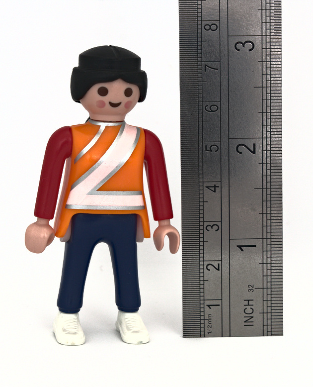
Back to playmobil

• height is a Ratio variable
• there will be limits to our precision, coventionally indicated by number of digits

height of figure (cm)

written	⊢ min	⊢ max
7.5	≥ 7.450	< 7.550
7.50	≥ 7.495	< 7.505

Histograms

• we can represent all the measurements with a histogram

• the bars are touching because this represents continuous data

Histograms

• we can represent all the measurements with a histogram

• the bars are touching because this represents continuous data

• we know that there were 7 measurements of about 7.50 cm
  • strictly, ≥ 7.495 and < 7.505 cm

Histograms (2)

• note that the bin width of the histogram matters

• these histograms all show the same data

Histograms in R

head(heights)

[1] 7.482 7.569 7.424 7.530 7.501 7.516

hist(heights)

you can make prettier graphs using ggplot(), but hist() is useful for exploring data

Histograms

the good

• way to examine the distribution of data

• easy to interpret (\(y\) axis = counts)

• sometimes helpful in spotting weird data

the bad

• changing bin width can completely change graph

• only gives info about distribution and mode

  • not, e.g., mean or median

Histograms

 [1] 7.504 4.196 7.516 7.385 7.550 7.500 7.473 7.453 7.424 7.583 7.445 7.609
[13] 7.502 7.466 7.531 7.425 7.546 7.452 7.490 7.463 7.473 7.481 7.580 7.544
[25] 7.482 4.199 7.628 7.489 7.560 7.471 7.488 7.503 7.507 7.406 7.500 7.565
[37] 7.466 7.394 7.509 7.522 7.462 7.529 7.567 7.461 7.514 7.474 7.532 7.530
[49] 7.462 7.508 7.569 7.539 7.566 7.447 7.486 7.627 7.501 7.487 7.539 7.513
[61] 7.581 7.522 7.529 7.500 7.491 7.523 7.485 7.527 7.412 7.560 7.512 7.650

Density Plots

• density plots depend on a smoothing function

• essentially, they’re making guesses where there is no data

Density Plots

• \(y\) axis is no longer a count
• total area under curve = “all possibilities” = 1

Density Plots

• partial area under the curve gives proportion of cases (here, 0.1885 ≥ 7.500 and < 7.525)

this is equivalent to saying that if I pick an observation \(x_i\) from this sample at random, there is a probability of .1885 that \(7.500 \le x_i < 7.525\)

The Normal Distribution

A Famous Density Plot

• when we started thinking about measurement, we thought things might look a bit like this

• the so-called normal curve

the normal curve is a hypothetical, asymptotic, density plot, with an area under the curve of 1

• in part 3, we’ll look at where the normal curve comes from

• for now, let’s look at some of its features

Normal Curves: Mean

• normal curves can be defined in terms of two parameters

• one is the centre or mean of the distribution (\(\bar{x}\), or sometimes \(\mu\))

• the y value here is just what is needed to ensure that the area under the is 1

Standard Deviation

• the other is the standard deviation (sd, or sometimes \(\sigma\))

\[\textrm{sd}=\sqrt{\frac{\sum{(x-\bar{x})^2}}{n-1}}\]

• standard deviation is the “average distance of observations from the mean”

Why Does the Height Vary?

• area under the curve is always the same by sd

• for ± 1 sd it’s 0.6827

there is a 68% chance of obtaining data within 1 sd of the mean

• remember though that we’re in hypothetical world!

The Standard Normal Curve

• we can standardize any value on any normal curve by

• subtracting the mean

  • the effective mean is now zero

• dividing by the standard deviation

  • the effective standard deviation is now one

\[ z_i = \frac{x_i - \bar{x}}{\sigma} \]

The Standard Normal Curve

• the area between 1 standard deviation below the mean and 1 standard deviation above the mean is, as we know, 0.6827

• we can ask the question the other way around: an area of .95 lies between -1.96 and 1.96 standard deviations from the mean

95% of the hypothetical observations (95% confidence interval)

⇢

Samples

Samples vs Populations

• population: all members of group you are hypothesizing about

• sample: the subset of the population you’re testing

Central Limit Theorem

• lay version: sample means will be normally distributed about the true mean

• if we repeatedly sample from a population, we’ll get a normal distribution of means

• the mean of the distribution of means will be (close to) the population mean

the standard deviation (“width”) of the distribution of sample means is referred to as the standard error of the distribution

Central Limit Theorem (2)

• if you look up CLT on Wikipedia you’ll see it’s defined in terms of adding two numbers

  • the sample mean is a sum of many numbers, divided by \(n\)

  • adding many numbers is like adding two numbers:

  \[\color{red}{1 + 3 + 2} + 5 = \color{red}{(1 + 3 + 2)} + 5 = \color{red}{6} + 5\]

  • dividing by something doesn’t make any difference

\(n-1\)

• we’ve just shown how adding many numbers is equivalent to adding two numbers

• so if we know the sum of a bunch of numbers, \(n-1\) of those numbers can be anything

sum of n-1 numbers	nth number	sum
90	10	100
102	-2	100
67	33	100

• so if we know a summary statistic (e.g., mean, sd) we know about the data with \(n-1\) degrees of freedom

Putting it Together

• the normal curve is a density plot with known properties

  • it can be defined in terms of two parameters: mean, and standard deviation

• if we repeatedly sample from a population and measure the mean, we’ll get a normal distribution

  • the mean of means will be (close to) the population mean

  • the standard deviation of the sample means is called the standard error

• if we don’t know the population, we’ll have to estimate the population mean

• we’ll want some kind of way of assessing how good our estimate is

Experiments (Unknown Population)

• in an experiment, we have access to a sample but not the population

• we have to estimate the population mean

Sample Estimates

• the estimated mean is the sample mean (we have no other info)

• the estimated standard error of the mean is defined in terms of the sample standard deviation

\[ \textrm{se} = \frac{\sigma}{\sqrt{n}} = \frac{\sqrt{\frac{\sum{(x-\bar{x})^2}}{n-1}}}{\sqrt{n}} \]

\[ \textrm{se} = \frac{\sigma}{\color{red}{\sqrt{n}}} = \frac{\sqrt{\frac{\sum{(x-\bar{x})^2}}{n-1}}}{\color{red}{\sqrt{n}}} \]

• the larger the sample size, the smaller the standard error

Confidence Intervals

• there is only one population mean

• our best estimate is the sample mean

• we know that 95% of our best estimates will fall within ±1.96 standard errors of the sample mean

• we have 95% confidence that our estimation technique will capture the true mean within ±1.96 standard errors

Can We Use This For Real?

• we have some survey data from the last couple of USMR classes, including height in cm

• perhaps we’re interested in the “mean height of a young statistician” (!)

  • “young statisticians” are a population

  • the USMR classes are a sample

can we use the information from the sample of 304 responses we have to say anything about the population?

Looking at the Class Data

# the class heights are
# in uheights
hist(uheights, xlab = "height (cm)")

• histogram suggests that the heights are (approximately) normally distributed

survey data from google forms can be read in directly with the {googlesheets4} library

Mean, Standard Deviation

• information about the distribution of the sample

mean(uheights)

[1] 167.9

sd(uheights)

[1] 8.755

Standard Error

• standard error is the “standard deviation of the mean”

• as we saw in the simulation

• can be estimated as \(\frac{\sigma}{\sqrt{n}}\)

n <- length(uheights)
# standard error
sd(uheights)/sqrt(n)

[1] 0.5021

Statistically Useful Information

• we know that the area between \(\bar{x}-1.96\sigma\) and \(\bar{x}+1.96\sigma\) is 0.95

based our sample of 304 people from the USMR class, we are 95% confident that the population mean lies between 166.9cm and 168.9cm

Statistically Useful Information

• we also have information from 3 other statistics courses

course	mean	se	n
dapr1	168.0	0.6780	118
dapr2	167.0	1.1239	48
rms2	167.4	0.9750	67
usmr	167.9	0.5021	304

• are the young statisticians on those courses from different populations? (in terms of height)

survey |> group_by(course) |> summarise(mean=mean(height),se=sd(height)/sqrt(n()), n=n())

Standard Errors (again)

USMR

\(\bar{x}=167.9\)

\(\text{se}=0.50\)

DAPR2

\(\bar{x}=167.0\)

\(\text{se}=1.12\)

Statistical Inference

• not much evidence that DAPR2 and USMR come from different populations

• inferring from samples to populations is a major goal of statistics

• more about this next time

End