Scaling and Contrasts

Univariate Statistics and Methodology using R

Martin Corley

Psychology, PPLS

University of Edinburgh

Scaling

Learning to Read

age	hrs_wk	method	R_AGE
9.982	5.137	phonics	14.090
8.006	4.353	phonics	11.762
9.349	5.808	phonics	13.838
8.678	5.441	phonics	13.315
10.150	4.589	phonics	14.271
10.454	4.605	word	9.634
9.366	4.612	word	7.981
8.620	3.612	word	6.620
8.060	4.447	word	7.524
6.117	5.085	word	5.502

Learning to Read

...
            Estimate Std. Error t value Pr(>|t|)  
(Intercept)    0.518      2.422    0.21    0.832  
age            0.578      0.222    2.61    0.012 *
hrs_wk         0.945      0.406    2.33    0.024 *
...

Learning to Read

...
            Estimate Std. Error t value Pr(>|t|)  
(Intercept)    0.518      2.422    0.21    0.832  
age            0.578      0.222    2.61    0.012 *
hrs_wk         0.945      0.406    2.33    0.024 *
...

• as we noted last week, the intercept for this model is nonsensical

  • “children aged zero who read for zero hours a week have a predicted reading age of 0.52”

• perhaps there’s something we can do about this?

One-Predictor Model

• let’s start with a model with a single predictor of age

# model
mod2 <- lm(R_AGE ~ age,
    data = reading)

# figure
reading |>
    ggplot(aes(x = age,
        y = R_AGE)) + xlab("age (yrs)") +
    ylab("reading age (yrs)") +
    geom_point(size = 3) +
    geom_smooth(method = "lm")

we know this model doesn’t meet assumptions, but it will work for an illustration

Changing the Intercept

• actually it’s fairly easy to move the intercept

• we can just pick a “useful-looking” value

• for example, we might want the intercept to tell us about students at age 8

  • this is a decision; no magic about it

Changing the Intercept

• actually it’s fairly easy to move the intercept

• we can just pick a “useful-looking” value

• for example, we might want the intercept to tell us about students at age 8

  • this is a decision; no magic about it

A Model With a New Intercept

original model

...
            Estimate Std. Error t value Pr(>|t|)   
(Intercept)    4.238      1.904    2.23   0.0307 * 
age            0.699      0.225    3.10   0.0032 **
...

new model

mod2b <- lm(R_AGE ~ I(age-8), data=reading)
summary(mod2b)

...
            Estimate Std. Error t value Pr(>|t|)    
(Intercept)    9.829      0.382    25.7   <2e-16 ***
I(age - 8)     0.699      0.225     3.1   0.0032 ** 
...

Fit Remains Unchanged

original model

...
Multiple R-squared:  0.167, Adjusted R-squared:  0.15 
F-statistic: 9.62 on 1 and 48 DF,  p-value: 0.00323

new model

...
Multiple R-squared:  0.167, Adjusted R-squared:  0.15 
F-statistic: 9.62 on 1 and 48 DF,  p-value: 0.00323

A Model with a New Slope

• it’s also easy to linearly scale the slope

• we can just pick a “useful” scale

• for example, we might want to examine the effect per month of age

  • this is a decision; no magic about it

A Model with a New Slope

• it’s also easy to linearly scale the slope

• we can just pick a “useful” scale

• for example, we might want to examine the effect per month of age

  • this is a decision; no magic about it

A Model With a New Slope

original model

...
            Estimate Std. Error t value Pr(>|t|)   
(Intercept)    4.238      1.904    2.23   0.0307 * 
age            0.699      0.225    3.10   0.0032 **
...

new model

mod2c <- lm(R_AGE ~ I(age*12), data=reading)
summary(mod2c)

...
            Estimate Std. Error t value Pr(>|t|)   
(Intercept)   4.2385     1.9037    2.23   0.0307 * 
I(age * 12)   0.0582     0.0188    3.10   0.0032 **
...

Fit Remains Unchanged

original model

...
Multiple R-squared:  0.167, Adjusted R-squared:  0.15 
F-statistic: 9.62 on 1 and 48 DF,  p-value: 0.00323

new model

...
Multiple R-squared:  0.167, Adjusted R-squared:  0.15 
F-statistic: 9.62 on 1 and 48 DF,  p-value: 0.00323

We Can Get Fancy About This

mod.mb <- lm(R_AGE ~ I((age-8)*12) + I(hrs_wk-mean(hrs_wk)), data=reading)
summary(mod.mb)

Call:
lm(formula = R_AGE ~ I((age - 8) * 12) + I(hrs_wk - mean(hrs_wk)), 
    data = reading)

Residuals:
   Min     1Q Median     3Q    Max 
-3.820 -2.382  0.074  2.404  3.549 

Coefficients:
                         Estimate Std. Error t value Pr(>|t|)    
(Intercept)                9.8627     0.3657   26.97   <2e-16 ***
I((age - 8) * 12)          0.0482     0.0185    2.61    0.012 *  
I(hrs_wk - mean(hrs_wk))   0.9455     0.4056    2.33    0.024 *  
---
Signif. codes:  0 '***' 0.001 '**' 0.01 '*' 0.05 '.' 0.1 ' ' 1

Residual standard error: 2.55 on 47 degrees of freedom
Multiple R-squared:  0.253, Adjusted R-squared:  0.221 
F-statistic: 7.97 on 2 and 47 DF,  p-value: 0.00105

But We Need to Know What We’re Doing

(Intercept)                9.8627     0.3657   26.97   <2e-16 ***

• model reading age of someone

  • aged 8
  • who reads for an average amount of hours/week

I((age - 8) * 12)          0.0482     0.0185    2.61    0.012 *  

• model increase in reading age per month of age

I(hrs_wk - mean(hrs_wk))   0.9455     0.4056    2.33    0.024 *  

• model increase in reading age per hour/wk of reading

• note that we need to understand all other coefficients in order to interpret intercept

Which Has a Bigger Effect?

• in our two-predictor model, is age more important than practise? Or vice-versa?

• hard to tell because the predictors are in different units

...
            Estimate Std. Error t value Pr(>|t|)  
(Intercept)    0.518      2.422    0.21    0.832  
age            0.578      0.222    2.61    0.012 *
hrs_wk         0.945      0.406    2.33    0.024 *
...

Standardisation

• if the predictors and outcome are very roughly normally distributed…

• we can calculate z-scores by subtracting the mean and dividing by the standard deviation

\[z_i=\frac{x_i-\bar{x}}{\sigma_x}\]

Standardisation

• in R, the scale() function calculates z-scores

• in R, you don’t need to create new columns

  • I() not obligatory because no ambiguity

mod.ms <- lm(scale(R_AGE) ~ scale(age) + scale(hrs_wk), data=reading)

Standardisation

• in R, the scale() function calculates z-scores

• in R, you don’t need to shouldn’t often create new columns

  • I() not obligatory because no ambiguity

mod.ms <- lm(scale(R_AGE) ~ scale(age) + scale(hrs_wk), data=reading)

• variables all in terms of standard deviations from the mean

• at the intercept, age and hrs_wk are at their means

• slopes: “how many standard deviations does R_AGE change for a one standard deviation change in the predictor?”

• model fit won’t change

Standardisation

summary(mod.ms)

...
              Estimate Std. Error t value Pr(>|t|)  
(Intercept)   2.39e-16   1.25e-01    0.00    1.000  
scale(age)    3.38e-01   1.30e-01    2.61    0.012 *
scale(hrs_wk) 3.02e-01   1.30e-01    2.33    0.024 *
...

• R_AGE changes 0.34 sds for a 1-sd change in age, and 0.30 sds for a 1-sd change in hrs_wk

• reasonable conclusion might be that age has a greater effect on reading age than does practice

• we expect the intercept to be zero because it’s the mean of everything

you can read \(2.39\times 10^{-16}\) as \(0\), with computer rounding error

Categorical Predictors

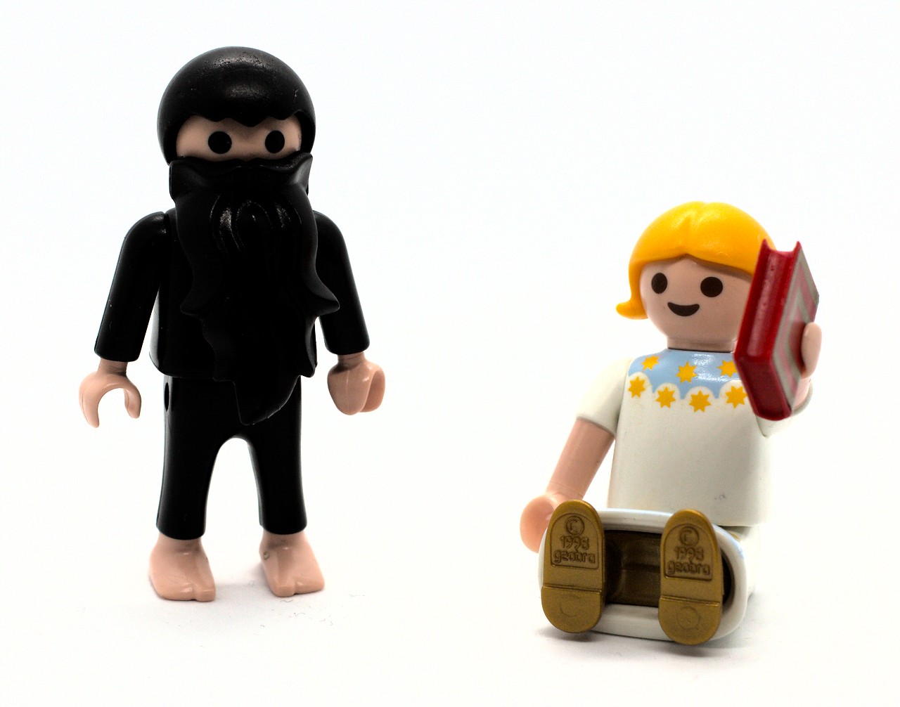
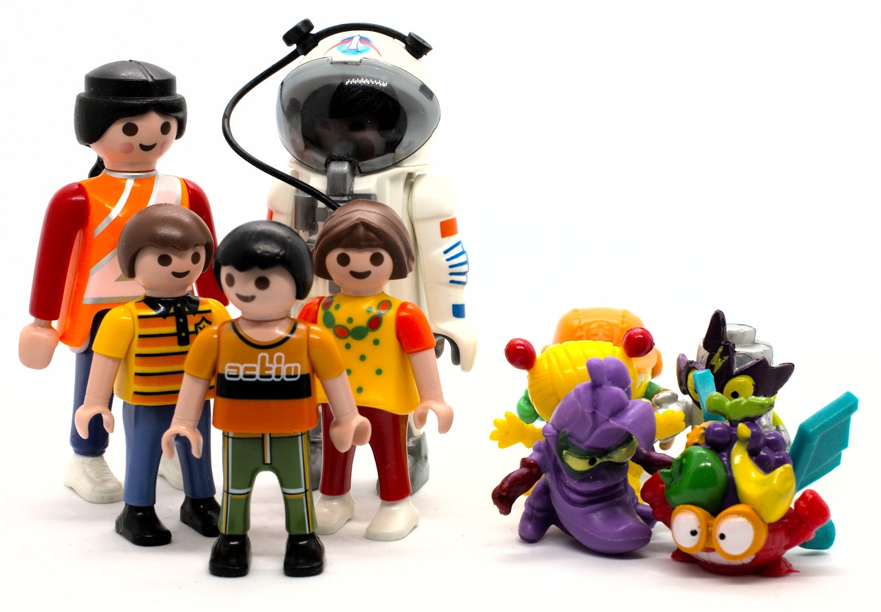
Playmobil vs. SuperZings

• some important pretesting went into these lectures

• every individual figure rated for “usefulness” in explaining stats

• how do we decide which to use?

Playmobil vs. SuperZings

type	UTILITY
playmo	9.7
zing	3.8
playmo	4.7
zing	0.1
playmo	5.1
zing	1.2
playmo	5.1
zing	2.1
playmo	2.5
zing	2.9

• we know one way to answer this

t.test(UTILITY ~ type, data = toys,
    var.equal = TRUE)

    Two Sample t-test

data:  UTILITY by type
t = 2.5, df = 8, p-value = 0.03
alternative hypothesis: true difference in means between group playmo and group zing is not equal to 0
95 percent confidence interval:
 0.3115 6.4885
sample estimates:
mean in group playmo   mean in group zing 
                5.42                 2.02 

The Only Equation You’ll Ever Need

• which toys are the most useful?

\[\color{red}{\textrm{outcome}_i}\color{white}=\color{blue}{(\textrm{model})_i}\color{white}{+\textrm{error}_i}\]

\[\color{red}{\textrm{utility}_i}\color{white}{=}\color{blue}{(\textrm{some function of type})_i}\color{white}{+\epsilon_i}\]

• we need to represent type as a number

• the simplest way of doing this is to use 0 or 1

Quantifying a Nominal Predictor

toys <- toys |>
    mutate(is_playmo = ifelse(type ==
        "playmo", 1, 0))
toys

# A tibble: 10 × 3
   type   UTILITY is_playmo
   <fct>    <dbl>     <dbl>
 1 playmo     9.7         1
 2 zing       3.8         0
 3 playmo     4.7         1
 4 zing       0.1         0
 5 playmo     5.1         1
 6 zing       1.2         0
 7 playmo     5.1         1
 8 zing       2.1         0
 9 playmo     2.5         1
10 zing       2.9         0

• this maps to a linear model

\[\color{red}{\textrm{utility}_i}=\color{blue}{b_0+b_1\cdot{}\textrm{is_playmo}}+\epsilon_i\]

• \(\overline{\textrm{utility}}\) for SuperZings is intercept

• “change due to playmo-ness” is slope

Linear Model Using is_playmo

mod1 <- lm(UTILITY ~ is_playmo, data = toys)
summary(mod1)

Call:
lm(formula = UTILITY ~ is_playmo, data = toys)

Residuals:
   Min     1Q Median     3Q    Max 
-2.920 -0.795 -0.320  0.680  4.280 

Coefficients:
            Estimate Std. Error t value Pr(>|t|)  
(Intercept)    2.020      0.947    2.13    0.065 .
is_playmo      3.400      1.339    2.54    0.035 *
---
Signif. codes:  0 '***' 0.001 '**' 0.01 '*' 0.05 '.' 0.1 ' ' 1

Residual standard error: 2.12 on 8 degrees of freedom
Multiple R-squared:  0.446, Adjusted R-squared:  0.377 
F-statistic: 6.44 on 1 and 8 DF,  p-value: 0.0348

• note that the \(t\) value (and the \(p\) value) are exactly what we got from our initial \(t\)-test

• the \(t\)-test is just a special case of the linear model

• in this specific (1 predictor, 2-level) case, F = t²

Let R Do the Work

contrasts(toys$type)

       zing
playmo    0
zing      1

• already built-in to factors

• NB the first value will be the default intercept (because \(b_n=0\) for that value)

  • can change this using the relevel() function (or tidyverse fct_relevel())

• as long as we have a factor, can just use lm() with that column

Linear Model Using type

original

summary(mod1)

...
(Intercept)    2.020      0.947    2.13    0.065 .
is_playmo      3.400      1.339    2.54    0.035 *
...

with the factor type

mod2 <- lm(UTILITY~type, data=toys)
summary(mod2)

...
(Intercept)    5.420      0.947    5.72  0.00044 ***
typezing      -3.400      1.339   -2.54  0.03479 *  
...

• why is the coefficient negative? why is the intercept different?

• point out the typezing label

Graphically

• shows “what the model is doing”, but isn’t a very good presentation

• the line suggests you can make predictions for types between playmo and zing

Graphically

• error bars represent one standard error of the mean

What About Lego Figures?

• we now have three groups

• can’t label them c(0, 1, 2) because that would express a linear relationship

Independent Effects

• “change due to lego-ness” is independent of other changes

• solution: add another predictor

toys <- toys |>
  mutate(
    is_playmo = ifelse(type == "playmo", 1, 0),
    is_lego = ifelse(type == "lego", 1, 0)
  )
head(toys)

# A tibble: 6 × 4
  type   UTILITY is_playmo is_lego
  <fct>    <dbl>     <dbl>   <dbl>
1 zing       3.8         0       0
2 playmo     9.7         1       0
3 lego       0.1         0       1
4 zing       0.1         0       0
5 playmo     4.7         1       0
6 lego       1.2         0       1

Three-Level Predictor: Two Coefficients

type	UTILITY	is_playmo	is_lego
zing	3.8	0	0
playmo	9.7	1	0
lego	0.1	0	1
zing	0.1	0	0
playmo	4.7	1	0
lego	1.2	0	1

\[\textrm{utility}_i=\color{blue}{b_0}\color{gray}{+b_1\cdot\textrm{is_playmo}_i+b_2\cdot\textrm{is_lego}_i}+\epsilon_i\]

\[\textrm{utility}_i=\color{blue}{b_0}\color{gray}{+b_1\cdot0+b_2\cdot0}+\epsilon_i\]

“utility of a zing”

Three-Level Predictor: Two Coefficients

type	UTILITY	is_playmo	is_lego
zing	3.8	0	0
playmo	9.7	1	0
lego	0.1	0	1
zing	0.1	0	0
playmo	4.7	1	0
lego	1.2	0	1

\[\textrm{utility}_i=\color{blue}{b_0}\color{red}{+b_1\cdot\textrm{is_playmo}_i}+\color{gray}{b_2\cdot\textrm{is_lego}_i}+\epsilon_i\] \[\textrm{utility}_i=\color{blue}{b_0}\color{red}{+b_1\cdot1}+\color{gray}{b_2\cdot0}+\epsilon_i\]

“change in utility from a zing due to being a playmo”

Three-Level Predictor: Two Coefficients

type	UTILITY	is_playmo	is_lego
zing	3.8	0	0
playmo	9.7	1	0
lego	0.1	0	1
zing	0.1	0	0
playmo	4.7	1	0
lego	1.2	0	1

\[\textrm{utility}_i=\color{blue}{b_0}\color{gray}{+b_1\cdot\textrm{is_playmo}_i}+\color{red}{b_2\cdot\textrm{is_lego}_i}+\epsilon_i\] \[\textrm{utility}_i=\color{blue}{b_0}\color{gray}{+b_1\cdot0}+\color{red}{b_2\cdot1}+\epsilon_i\]

“change in utility from a zing due to being a lego”

Three-level Predictor Linear Model

mod <- lm(UTILITY ~ is_playmo + is_lego, data = toys)
summary(mod)

Call:
lm(formula = UTILITY ~ is_playmo + is_lego, data = toys)

Residuals:
   Min     1Q Median     3Q    Max 
 -2.92  -0.77   0.04   0.49   4.28 

Coefficients:
            Estimate Std. Error t value Pr(>|t|)  
(Intercept)    2.020      0.792    2.55    0.025 *
is_playmo      3.400      1.120    3.04    0.010 *
is_lego       -0.860      1.120   -0.77    0.457  
---
Signif. codes:  0 '***' 0.001 '**' 0.01 '*' 0.05 '.' 0.1 ' ' 1

Residual standard error: 1.77 on 12 degrees of freedom
Multiple R-squared:  0.574, Adjusted R-squared:  0.503 
F-statistic:  8.1 on 2 and 12 DF,  p-value: 0.00595

Let R Do the Work

• what we saw was, conceptually, a multiple regression (two predictors)

contrasts(toys$type)

       playmo lego
zing        0    0
playmo      1    0
lego        0    1

• already built-in to factors, as before

• NB this time zing is the intercept

obviously I’ve changed the toys dataframe behind the scenes

Let R Do the Work

mod <- lm(UTILITY ~ type, data = toys)
summary(mod)

Call:
lm(formula = UTILITY ~ type, data = toys)

Residuals:
   Min     1Q Median     3Q    Max 
 -2.92  -0.77   0.04   0.49   4.28 

Coefficients:
            Estimate Std. Error t value Pr(>|t|)  
(Intercept)    2.020      0.792    2.55    0.025 *
typeplaymo     3.400      1.120    3.04    0.010 *
typelego      -0.860      1.120   -0.77    0.457  
---
Signif. codes:  0 '***' 0.001 '**' 0.01 '*' 0.05 '.' 0.1 ' ' 1

Residual standard error: 1.77 on 12 degrees of freedom
Multiple R-squared:  0.574, Adjusted R-squared:  0.503 
F-statistic:  8.1 on 2 and 12 DF,  p-value: 0.00595

Let R Do the Work

mod <- lm(UTILITY ~ type, data = toys)
summary(mod)

Call:
lm(formula = UTILITY ~ type, data = toys)

Residuals:
   Min     1Q Median     3Q    Max 
 -2.92  -0.77   0.04   0.49   4.28 

Coefficients:
            Estimate Std. Error t value Pr(>|t|)  
(Intercept)    2.020      0.792    2.55    0.025 *
typeplaymo     3.400      1.120    3.04    0.010 *
typelego      -0.860      1.120   -0.77    0.457  
---
Signif. codes:  0 '***' 0.001 '**' 0.01 '*' 0.05 '.' 0.1 ' ' 1

Residual standard error: 1.77 on 12 degrees of freedom
Multiple R-squared:  0.574, Adjusted R-squared:  0.503 
F-statistic:  8.1 on 2 and 12 DF,  p-value: 0.00595

\[\hat{\textrm{utility}}= b_0\]

Let R Do the Work

mod <- lm(UTILITY ~ type, data = toys)
summary(mod)

Call:
lm(formula = UTILITY ~ type, data = toys)

Residuals:
   Min     1Q Median     3Q    Max 
 -2.92  -0.77   0.04   0.49   4.28 

Coefficients:
            Estimate Std. Error t value Pr(>|t|)  
(Intercept)    2.020      0.792    2.55    0.025 *
typeplaymo     3.400      1.120    3.04    0.010 *
typelego      -0.860      1.120   -0.77    0.457  
---
Signif. codes:  0 '***' 0.001 '**' 0.01 '*' 0.05 '.' 0.1 ' ' 1

Residual standard error: 1.77 on 12 degrees of freedom
Multiple R-squared:  0.574, Adjusted R-squared:  0.503 
F-statistic:  8.1 on 2 and 12 DF,  p-value: 0.00595

\[\hat{\textrm{utility}}= b_0\]

\[+ \color{blue}{b_1} . \textrm{is_playmo}\]

Let R Do the Work

mod <- lm(UTILITY ~ type, data = toys)
summary(mod)

Call:
lm(formula = UTILITY ~ type, data = toys)

Residuals:
   Min     1Q Median     3Q    Max 
 -2.92  -0.77   0.04   0.49   4.28 

Coefficients:
            Estimate Std. Error t value Pr(>|t|)  
(Intercept)    2.020      0.792    2.55    0.025 *
typeplaymo     3.400      1.120    3.04    0.010 *
typelego      -0.860      1.120   -0.77    0.457  
---
Signif. codes:  0 '***' 0.001 '**' 0.01 '*' 0.05 '.' 0.1 ' ' 1

Residual standard error: 1.77 on 12 degrees of freedom
Multiple R-squared:  0.574, Adjusted R-squared:  0.503 
F-statistic:  8.1 on 2 and 12 DF,  p-value: 0.00595

\[\hat{\textrm{utility}} = b_0\]

\[+ \color{blue}{b_1}\cdot\textrm{is_playmo}\]

\[+ \color{red}{b_2}\cdot\textrm{is_lego}\]

Graphically

\[\textrm{utility}_i=\color{grey}{b_0}\color{blue}{+b_1}\cdot\textrm{is_playmo}_i+\color{red}{b_2}\cdot\textrm{is_lego}_i+\epsilon_i\]

Not Quite a Multiple Regression

anova(mod)

Analysis of Variance Table

Response: UTILITY
          Df Sum Sq Mean Sq F value Pr(>F)   
type       2   50.7   25.37     8.1 0.0059 **
Residuals 12   37.6    3.13                  
---
Signif. codes:  0 '***' 0.001 '**' 0.01 '*' 0.05 '.' 0.1 ' ' 1

• type is still one variable

• in some sense it can’t be decomposed

• but it has two degrees of freedom because \(b_1\) and \(b_2\) are independent of each other

End