Correlations

Univariate Statistics and Methodology using R

Martin Corley

Psychology, PPLS

University of Edinburgh

Correlation

Blood Alcohol and Reaction Time

• data from 100 drivers
• are blood alcohol and RT (linearly) related?

• the playmo crew have been out joyriding and were caught in a police speed trap

• the police measured 100 people’s blood alcohol and their reaction times

• how would we go about telling whether two variables like this were related?

A Simplified Case

• does \(y\) vary linearly with \(x\)?

• equivalent to asking “does \(y\) differ from its mean in the same way that \(x\) does?”

• here are the ways in which the values of \(x\) differ from mean(x)
• and here are the ways in which \(y\) varies from its mean

Covariance

• it’s likely the variables are related if observations differ proportionately from their means

Covariance

variance

\[ s^2 = \frac{\sum{(x-\bar{x})^2}}{n} = \frac{\sum{(x-\bar{x})(x-\bar{x})}}{n} \]

covariance

\[ \textrm{cov}(x,y) = \frac{\sum{\color{blue}{(x-\bar{x})}\color{red}{(y-\bar{y})}}}{n} \]

• here we’re using \(n\), not \(n-1\), because this is the whole population

• for any (x,y), \(x-\bar{x}\) might be positive and \(y-\bar{y}\) might be positive, so the covariance could be a negative number

Covariance

\(\color{blue}{x-\bar{x}}\)	\(\color{red}{y-\bar{y}}\)	\(\color{blue}{(x-\bar{x})}\color{red}{(y-\bar{y})}\)
-0.3	1.66	-0.5
0.81	2.21	1.79
-1.75	-2.85	4.99
-0.14	-3.58	0.49
1.37	2.56	3.52
		10.29

\[\textrm{cov}(x,y) = \frac{\sum{(x-\bar{x})(y-\bar{y})}}{n} = \frac{10.29}{5} \simeq \color{red}{2.06}\]

I’ve rounded the numbers at the end to make this a bit neater on the slide

The Problem With Covariance

miles

\(x-\bar{x}\)	\(y-\bar{y}\)	\((x-\bar{x})(y-\bar{y})\)
-0.3	1.66	-0.5
0.81	2.21	1.79
-1.75	-2.85	4.99
-0.14	-3.58	0.49
1.37	2.56	3.52
		10.29

\[\textrm{cov}(x,y)=\frac{10.29}{5}\simeq 2.06\]

kilometres

\(x-\bar{x}\)	\(y-\bar{y}\)	\((x-\bar{x})(y-\bar{y})\)
-0.48	2.68	-1.29
1.3	3.56	4.64
-2.81	-4.59	12.91
-0.22	-5.77	1.27
2.21	4.12	9.12
		26.65

\[ \textrm{cov}(x,y)=\frac{26.65}{5}\simeq 5.33 \]

• these are exactly the same ‘values’ so they should each be as correlated as the other

• so we need to divide covariance by something to represent the overall “scale” of the units

Correlation Coefficient (\(r\))

\[r = \frac{\textrm{covariance}(x,y)}{\textrm{standard deviation}(x)\cdot\textrm{standard deviation}(y)}\]

\[r=\frac{\frac{\sum{(x-\bar{x})(y-\bar{y})}}{n}}{\sqrt{\frac{\sum{(x-\bar{x})^2}}{n}}\sqrt{\frac{\sum{(y-\bar{y})^2}}{n}}}\]

\[r=\frac{\frac{\sum{(x-\bar{x})(y-\bar{y})}}{\color{red}{n}}}{\sqrt{\frac{\sum{(x-\bar{x})^2}}{\color{red}{n}}}\sqrt{\frac{\sum{(y-\bar{y})^2}}{\color{red}{n}}}}\]

\[r=\frac{\sum{(x-\bar{x})(y-\bar{y})}}{\sqrt{\sum{(x-\bar{x})^2}}\sqrt{\sum{(y-\bar{y})^2}}}\]

standardised covariance, ensuring that units have no effect

Correlation Coefficient

• measure of how related two variables are

• \(-1 \le r \le 1\) (\(\pm 1\) = perfect fit; \(0\) = no fit)

\[ r=0.4648 \]

\[ r=-0.4648 \]

• on the left, we have the drunken drivers from our first slide, and you can see that there is a moderate positive correlation
  • the higher your blood alcohol, the slower your RT
• on the right, we have a negative correlation: what the drivers think happens
  • the higher your blood alcohol, the faster your RT

What Does the Value of r Mean?

Significance

Significance of a Correlation

\[ r = 0.4648 \]

• the police have stopped our friends and measured their blood alcohol

• is their evidence sufficient to conclude that there is likely to be a relationship between blood alcohol and reaction time?

Significance of a Correlation

• we can measure a correlation using \(r\)

• we want to know whether that correlation is significant

  • i.e., whether the probability of finding it by chance is low enough

• cardinal rule in NHST: compare everything to chance

• let’s investigate…

Random Correlations

• pick some pairs of numbers at random, return correlation

• arbitrarily, I’ve picked numbers uniformly distributed between 0 and 100

x <- runif(5, min = 0, max = 100)
y <- runif(5, min = 0, max = 100)
cbind(x, y)

         x     y
[1,] 58.38 82.33
[2,] 77.90 17.03
[3,] 56.58 21.52
[4,] 47.06 27.70
[5,] 73.68 29.14

cor(x, y)

[1] -0.254

Random Correlations

• pick some pairs of numbers at random, return correlation

  • repeat 1000 times

randomCor <- function(size) {
    x <- runif(size, min = 0,
        max = 100)
    y <- runif(size, min = 0,
        max = 100)
    cor(x, y)  # calculate r
}

# then we can use the
# usual trick:
rs <- replicate(1000, randomCor(5))
hist(rs)

Random Correlations

Calculating Probability

• distribution of random \(r\)s is \(t\) distribution, with \(n-2\) df

\[t= r\sqrt{\frac{n-2}{1-r^2}}\]

• makes it “easy” to calculate probability of getting \(\ge{}r\) for sample size \(n\) by chance

Calculating Probability

calculate \(t\)

r_to_t <- function (r,n) {
  r * sqrt((n-2) / (1-r^2))
}

r_to_t(0.4648, 50)

[1] 3.637

calculate \(p\)

2 * pt(3.637, 48, lower.tail=F)

[1] 0.0006727

• note 2 * pt(...) as this is a two-tailed hypothesis

\[r=0.4648\]

or just be lazy

cor.test(dat$BloodAlc, dat$RT)

    Pearson's product-moment correlation

data:  dat$BloodAlc and dat$RT
t = 3.6, df = 48, p-value = 0.0007
alternative hypothesis: true correlation is not equal to 0
95 percent confidence interval:
 0.2141 0.6580
sample estimates:
   cor 
0.4648 

Correlation++

Back on the Road

\[r= 0.4648, p = 0.0007\]

reaction time is positively associated with blood alcohol

• not a very complete picture

• how much does alcohol affect RT?

The Only Equation You Will Ever Need

\[\color{red}{\textrm{outcome}_i} = (\textrm{model})_i + \textrm{error}_i\]

The Only Equation You Will Ever Need

\[\color{red}{\textrm{outcome}_i} = \color{blue}{(\textrm{model})_i} + \textrm{error}_i\]

The Only Equation You Will Ever Need

\[\color{red}{\textrm{outcome}_i} = \color{blue}{(\textrm{model})_i} + \textrm{error}_i\]

The Only Equation You Will Ever Need

\[\color{red}{\textrm{outcome}_i} = \color{blue}{(\textrm{model})_i} + \textrm{error}_i\]

The Aim of the Game

\[\color{red}{\textrm{outcome}_i} = \color{blue}{(\textrm{model})_i} + \textrm{error}_i\]

• maximise the explanatory worth of the model

• minimise the amount of unexplained error

• explain more than one outcome!

Many Outcomes

• so far, have been talking about the i^th observation

• we want to generalise (“for any i”)

\[\color{red}{\textrm{outcomes}}=\color{blue}{\textrm{(model)}}+\textrm{errors}\]

We need to make assumptions

• model is linear

• errors are from a normal distribution

A Linear Model

• defined by two properties

• height of the line (intercept)

• slope of the line

A Linear Model

\[\color{red}{\textrm{outcome}_i} = \color{blue}{(\textrm{model})_i} + \textrm{error}_i\] \[\color{red}{y_i} = \color{blue}{\textrm{intercept}\cdot{}1+\textrm{slope}\cdot{}x_i}+\epsilon_i\]

\[\color{red}{y_i} = \color{blue}{b_0 \cdot{} 1 + b_1 \cdot{} x_i} + \epsilon_i\] so the linear model itself is…

\[\hat{y}_i = \color{blue}{b_0 \cdot{} 1 + b_1 \cdot{} x_i}\]

\[\color{blue}{b_0=5}, \color{blue}{b_1=2}\] \[\color{orange}{x_i=1.2},\color{red}{y_i=9.9}\] \[\hat{y}_i=7.4\]

so we can see that for this particular datapoint \((x_i,y_i)\) the error is 2.5

A Linear Model

\[\hat{y}_i = \color{blue}{b_0 \cdot{}}\color{orange}{1} \color{blue}{+b_1 \cdot{}} \color{orange}{x_i}\]

• values of the linear model (coefficients)

• values we provide (inputs)

• maps directly to R “formula” notation

A Linear Model

\[\color{red}{\textrm{outcome}_i} = \color{blue}{(\textrm{model})_i} + \textrm{error}_i\] \[\color{red}{y_i} = \color{blue}{\textrm{intercept}}\cdot{}\color{orange}{1}+\color{blue}{\textrm{slope}}\cdot{}\color{orange}{x_i}+\epsilon_i\] \[\color{red}{y_i} = \color{blue}{b_0} \cdot{} \color{orange}{1} + \color{blue}{b_1} \cdot{} \color{orange}{x_i} + \epsilon_i\] so the linear model itself is…

\[\hat{y}_i = \color{blue}{b_0} \cdot{} \color{orange}{1} + \color{blue}{b_1} \cdot{} \color{orange}{x_i}\]

\[\hat{y}_i = \color{blue}{b_0} + \color{blue}{b_1} \cdot{} \color{orange}{x_i}\]

Back on the Road 2

• simplify the data to make interpretation easier

ourDat <- dat |>
  mutate(BloodAlc = BloodAlc * 100)

mod <- lm(RT ~ BloodAlc, data = ourDat)

note that there’s no output from the R command, we’ve just created a model for interrogation

multiplying blood alcohol values is simple scaling, which we’ll revisit

Linear Model Output

summary(mod)

Call:
lm(formula = RT ~ BloodAlc, data = ourDat)

Residuals:
    Min      1Q  Median      3Q     Max 
-115.92  -40.42    1.05   42.93  126.64 

Coefficients:
            Estimate Std. Error t value Pr(>|t|)    
(Intercept)   321.24      91.05    3.53  0.00093 ***
BloodAlc       32.28       8.88    3.64  0.00067 ***
---
Signif. codes:  0 '***' 0.001 '**' 0.01 '*' 0.05 '.' 0.1 ' ' 1

Residual standard error: 55.8 on 48 degrees of freedom
Multiple R-squared:  0.216, Adjusted R-squared:   0.2 
F-statistic: 13.2 on 1 and 48 DF,  p-value: 0.000673

Possibly Back on the Road

for every extra 0.01% blood alcohol, reaction time slows down by around 32 ms

• remember that one unit is 0.01%, because we multiplied by 100

Significance

The Null Hypotheses

• b₀ won’t be significantly different from zero

  • not (always) interesting

• b₁ won’t be significantly different from zero

  • “knowing x doesn’t tell you anything about y”

Let’s Simulate!

Many Regressions

Significance

• we’ve already seen something in the model summary

summary(mod)

...
Coefficients:
            Estimate Std. Error t value Pr(>|t|)    
(Intercept)   321.24      91.05    3.53  0.00093 ***
BloodAlc       32.28       8.88    3.64  0.00067 ***
...

• the logic is the same as for \(t\) tests

• \(t\) value is \(\frac{\textrm{estimate}}{\textrm{standard error}}\)

• standard errors are calculated from model like for \(t\)-tests

Degrees of Freedom

• let’s talk about DF

• here are random collections of 8 datapoints

• each graph has 8 points, each graph has a line of best fit

• now, for these collections of 8 points,

• we can always add in another two points to each plot and make the best fit line the same in each

Degrees of Freedom

• so here we’ve added two points to each, and the lines are now the same in each

• this is one way of showing that for \(n\) data points, there are \(n-2\) degrees of freedom

Degrees of Freedom

• we subtract 2 df because we “know” two things

  • intercept (b₀)

  • slope (b₁)

• the remaining df are the residual degrees of freedom

...
BloodAlc       32.28       8.88    3.64  0.00067 ***
...
F-statistic: 13.2 on 1 and 48 DF,  p-value: 0.000673

reaction time slowed by 32.3 ms for every additional 0.01% blood alcohol by volume (t(48)=3.64, p=.0007)

• we subtract 2, because we know 2 things - the intercept and the slope.
• the remaining degrees of freedom are residual degrees of freedom
• and our tests of intercept and slope will be calculated using t distribution with 18 df

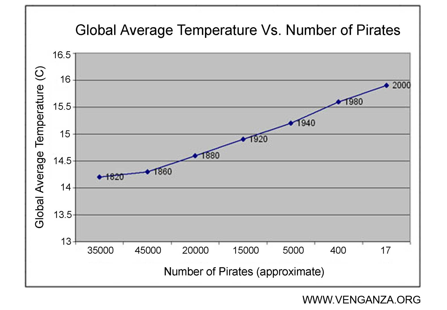
Pirates and Global Warming