Introductions to R and Statistics

Univariate Statistics and Methodology using R

Martin Corley

Psychology, PPLS

University of Edinburgh

Five Things to Do

1. watch the introductory lecture on Learn

2. find piazza on Learn, and introduce yourself

3. get the software (or check that rstudio.ppls.ed.ac.uk works for you)

4. fill in the survey at edin.ac/3B0oi5A

5. check what lab you’re in (bring a charged laptop if possible)

Why R?

What is R?

• R is a ‘statistical programming language’

• created mid-90s as a free version of S

• widespread adoption since v2 (2004)

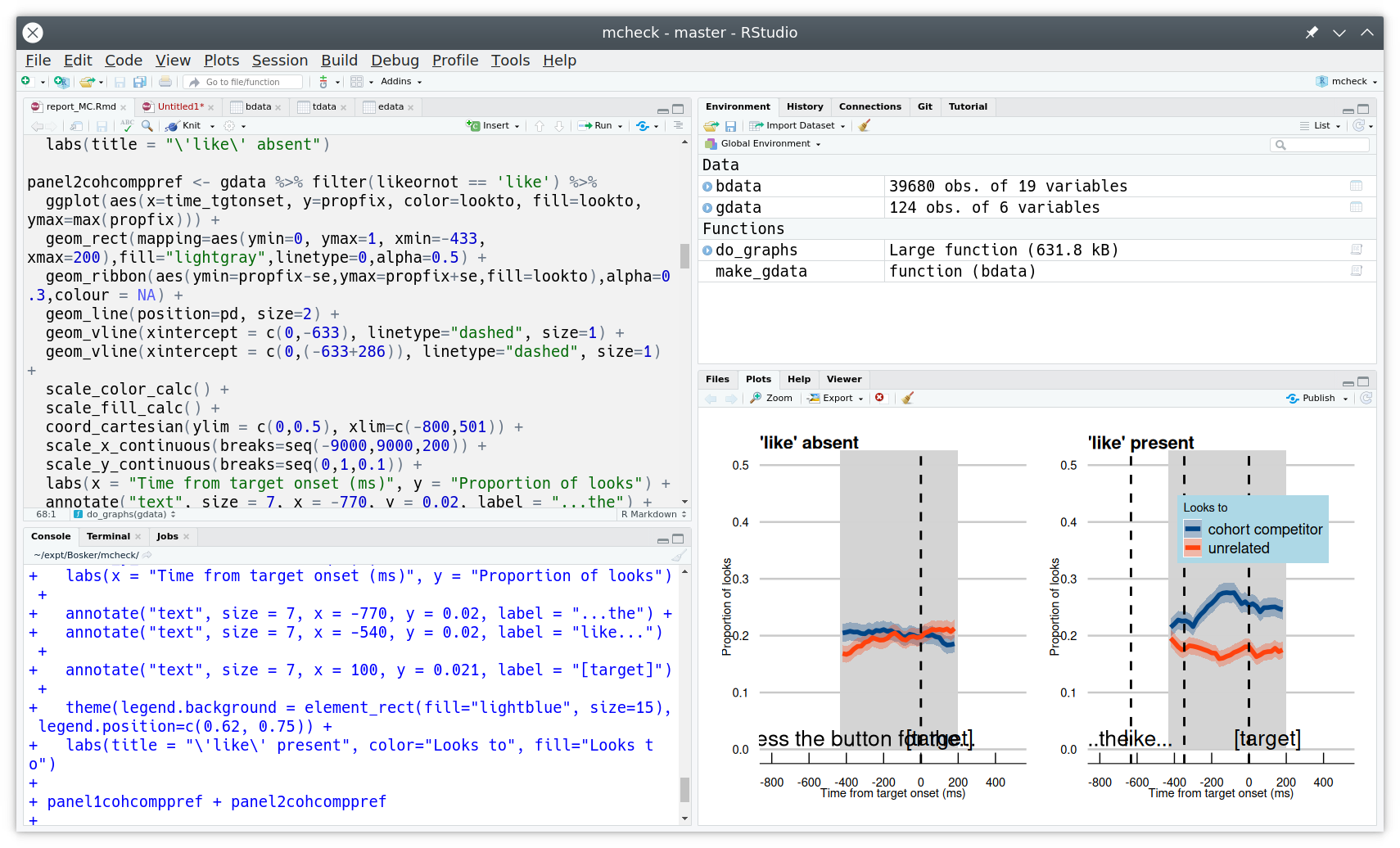
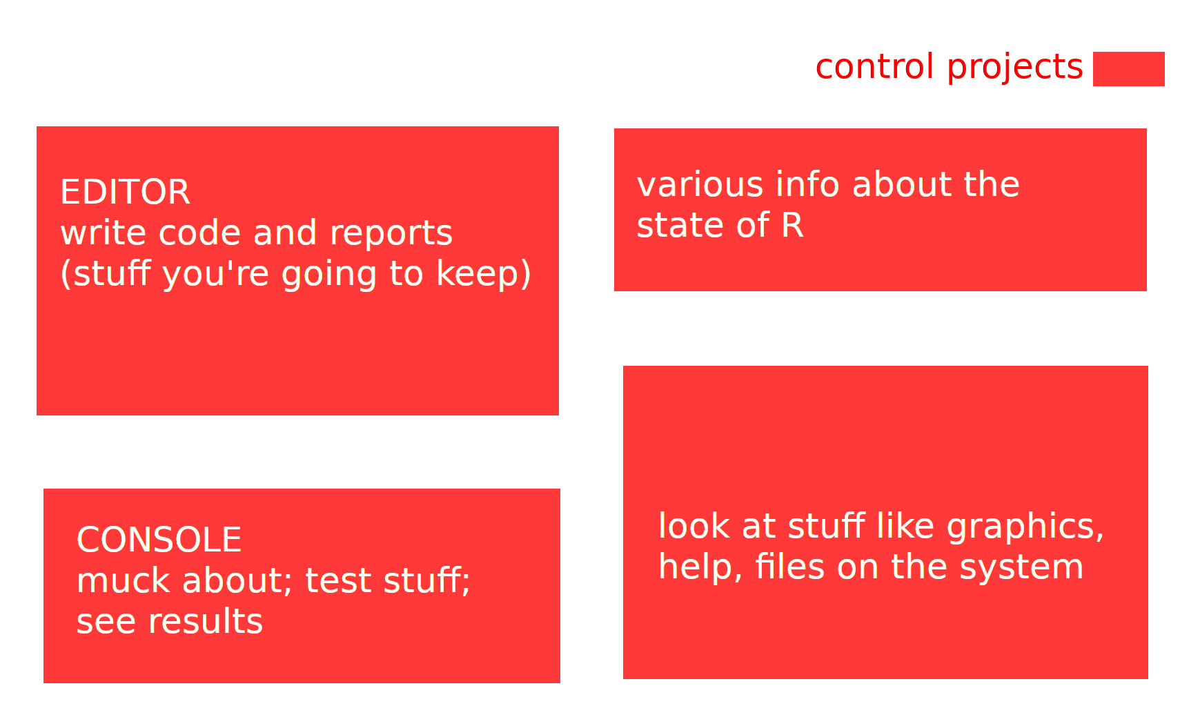
• RStudio is an ‘integrated development environment’ (IDE)

• created 2011 ‘to improve R experience’

• widespread adoption since 2012

R vs RStudio

This is R

model <- lm(RT ~ (age+freq+handedness)^2, data=words)
summary(model)

This is RStudio

RMarkdown

• RMarkdown is a ‘text markup language’

• created 2012 as a markup language for R

• widespread adoption since 2015

• Quarto is the latest-and-greatest RMarkdown version

• the one to learn if you want to get serious

RMarkdown

### About RMarkdown

_This_ is some **RMarkdown**, which uses 'simple' codes to mark up text.

- it can include R code like `r sqrt(2)`
- it's simple to format things like bulleted lists
  + or even sublists

About RMarkdown

This is some RMarkdown, which uses ‘simple’ codes to mark up text.

• it can include R code like 1.4142
• it’s simple to format things like bulleted lists
  • or even sublists

What is R Good For?

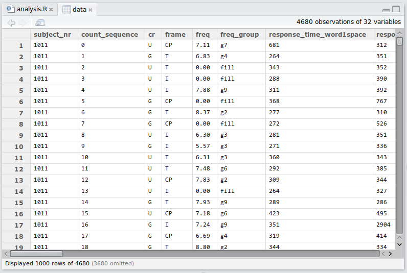
Managing Datasets

Doing Statistics

Generalized linear mixed model fit by maximum likelihood (Laplace
  Approximation) [glmerMod]
 Family: binomial  ( logit )
Formula: DV ~ sc(FvO) * sc(EvC) + (1 | Code) + (0 + (sc(FvO) * sc(EvC)) |  
    Code) + (1 | Item)
   Data: feminine
Control: glmerControl(optimizer = "bobyqa")

     AIC      BIC   logLik deviance df.resid 
   879.3    943.6   -427.7    855.3     1558 
...
Fixed effects:
                Estimate Std. Error z value Pr(>|z|)    
(Intercept)      -1.0566     1.1485   -0.92  0.35758    
sc(FvO)           1.2453     0.3505    3.55  0.00038 ***
sc(EvC)          -0.0915     0.3080   -0.30  0.76638    
sc(FvO):sc(EvC)   0.0221     0.6321    0.04  0.97207    
---
Signif. codes:  0 '***' 0.001 '**' 0.01 '*' 0.05 '.' 0.1 ' ' 1
...

Publication-Quality Graphics

Data Visualisation

https://www.facebook.com/notes/10158791468612200/

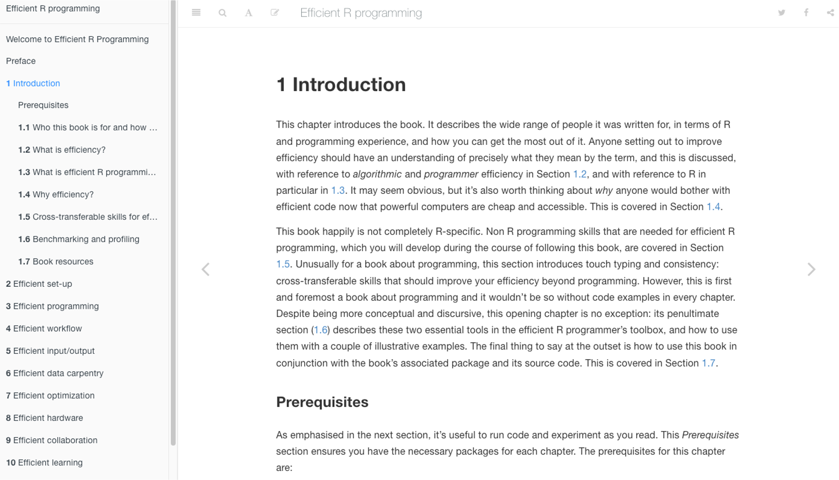
RMarkdown: Books

https://bookdown.org/csgillespie/efficientR/

RMarkdown: Websites

https://martincorley.org/

Online Interactive Visualisation

https://shiny.posit.co/r/gallery/interactive-visualizations/movie-explorer/

R for Anything to do with Data

require(tm)
require(wordcloud)
pp <- Corpus(DirSource("R/PP/"))
pp <- tm_map(pp, stripWhitespace)
pp <- tm_map(pp, tolower)
pp <- tm_map(pp, removeWords,
    stopwords("english"))
pp <- tm_map(pp, stemDocument)
pp <- tm_map(pp, removePunctuation)
pp <- tm_map(pp, PlainTextDocument)
wordcloud(pp, scale = c(5,
    0.5), max.words = 150,
    random.order = FALSE,
    rot.per = 0.35, colors = brewer.pal(12,
        "Dark2"))

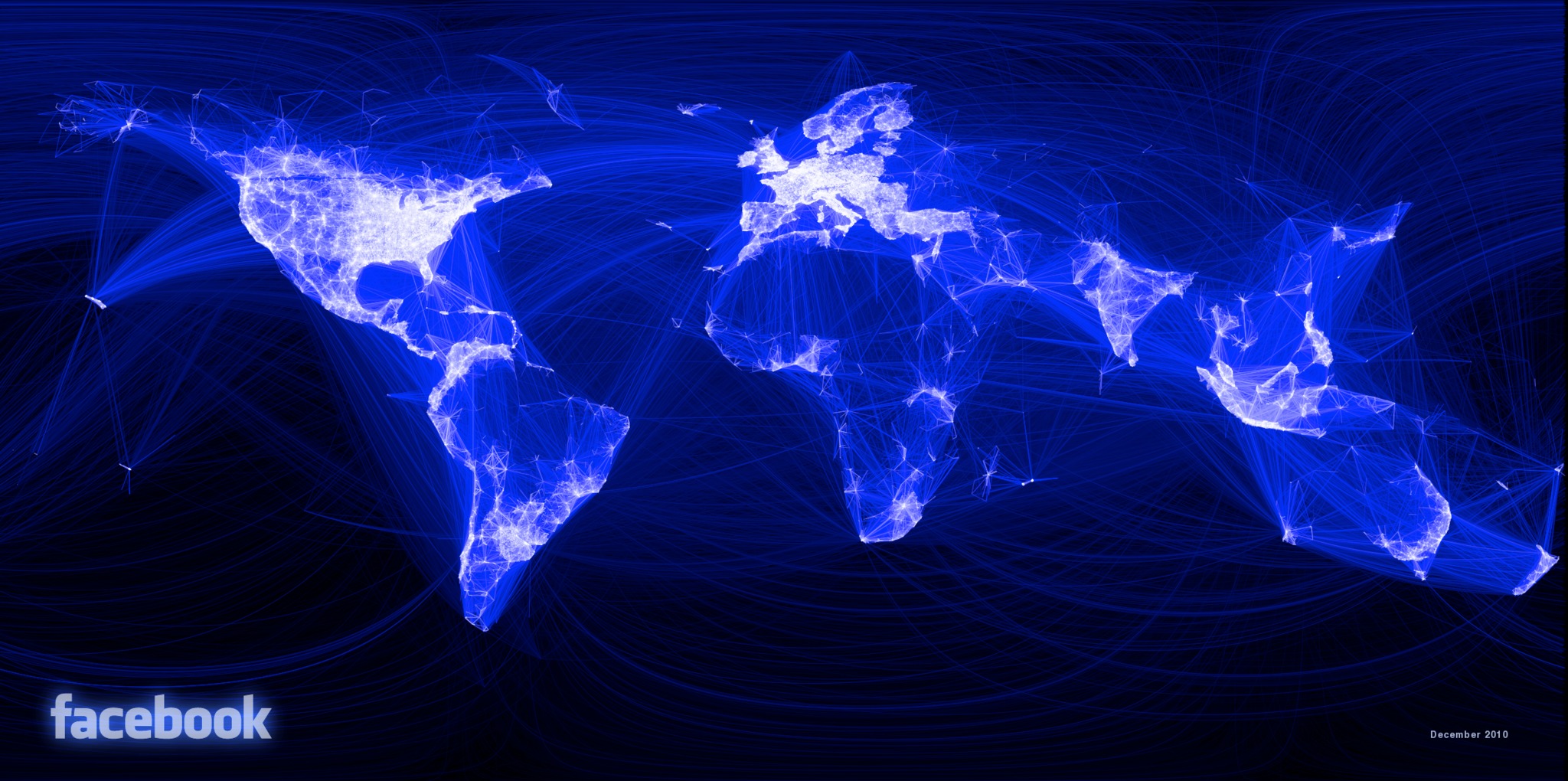
The R Community

• someone else has done all the hard work to create wordclouds
• released as libraries or packages (like lme4 and tidyverse)
• all I supplied was a text version of Pride and Prejudice

• R allows you to do anything with data
• if it’s useful, chances are someone has already done it
• useful things include statistics!

The R Community

• if it’s useless, chances are that someone’s already done it

library(cowsay)
say("hello USMR")

 -------------- 
hello USMR 
 --------------
    \
      \
        \
            |\___/|
          ==) ^Y^ (==
            \  ^  /
             )=*=(
            /     \
            |     |
           /| | | |\
           \| | |_|/\
      jgs  //_// ___/
               \_)
  

• USMR is created in RStudio, using R and RMarkdown

Why Use R?

• because it’s a language, I can easily show you what I did and you can copy it

• because it’s a language, statisticians can use it to implement leading-edge stats

• because it’s free, anyone can use it—and anyone can access your research

• because it’s open source, anyone can fix or improve it

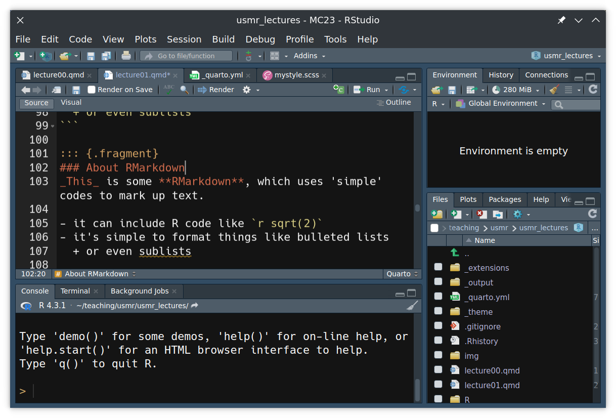
Devilish Stuff

doing stats

coding

 

this is the first note for wizards

all indices in R start at 1

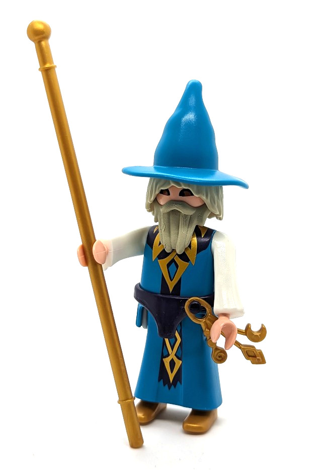
Notes for Wizards

• did you notice my hat on the last slide?

• it marks something that’s good to know but you don’t need to know (yet)

• “notes for wizards” (of all genders and none!)

these photos were taken using a cheap (£12) lightbox

Basics of R

Data in R

• you can type data directly in to R

# a number
1.2

[1] 1.2

# characters (a string)
"fáilte"

[1] "fáilte"

• and you can do operations on data

1.2 + 7 * 2

[1] 15.2

• why is the answer 15.2 and not 16.4?
• by “data” we really mean anything that is measured outside R and provided to R directly

Variables

• you can assign data to variables

bodyTemp <- 37.8

• and use those variables

bodyTemp * (9/5) + 32  # to Fahrenheit

[1] 100

• NB spelling/capitalization matter

BodyTemp - 37

Error in eval(expr, envir, enclos): object 'BodyTemp' not found

Statistics is about Groups

allTemps <- c(37.8, 0, 37.4)

# vector maths
allTemps * (9/5) + 32

[1] 100.04  32.00  99.32

• note the vectorization of the calculation

• R is designed from the bottom up to deal with groups

Not everything is a number

allHair <- c("brown", "white", "black")
allHair

[1] "brown" "white" "black"

• these are called character strings
  • can be anything
• categories (nominal data) are from a limited set
  • called factors in R

as.factor(allHair)

[1] brown white black
Levels: black brown white

Basic types of data (stats)

• Nominal

  (‘names of things’: e.g., hair colour)

• Ordinal

  (order, no number: e.g., small-medium-large)

• Interval

  (number without a true zero: e.g., body temp in ℃)

• Ratio

  (number with a true zero: e.g., height)

NOIR in R

Type	R Variable Type
Nominal	character/factor
Ordinal	number
Interval	number
Ratio	number

• nominal

allHair <- as.factor(c("brown", "white",
    "black"))
allHair

[1] brown white black
Levels: black brown white

• interval

allTemps <- c(37.8, 0, 37.4)
allTemps

[1] 37.8  0.0 37.4

ordinal data can also be represented as ordered factors (as.ordered())

Break it down

allHair <- c("brown", "white", "black")

 

allHair

• variable (we chose the name allHair)

<-

• assignment (“goes in to”)

c()

• function (c() combines its arguments)

"brown"

• character (arbitrary sequence of symbols)

• only the middle two are “R”; the others are strings we chose.

Dataframes

• data can be grouped into a dataframe
• each line represents one set of observations
• each column represents one type of information
  • (a bit like a spreadsheet)

people <- data.frame(
  name = c("Johanna", "Casper", "Steve"),
  temp = allTemps, hair = as.factor(allHair),
  height = c(132, 205, 181)
)
people

     name temp  hair height
1 Johanna 37.8 brown    132
2  Casper  0.0 white    205
3   Steve 37.4 black    181

• note that I’ve made hair a factor but left names as character strings.

• that’s because, in my world, there is a finite set of hair colours, but a name can be anything: it’s an arbitrary label.

• you’ll see the effect of this in the next slide.

Functions and dataframes

• you can run a function on a dataframe

summary(people)

     name                temp         hair       height   
 Length:3           Min.   : 0.0   black:1   Min.   :132  
 Class :character   1st Qu.:18.7   brown:1   1st Qu.:156  
 Mode  :character   Median :37.4   white:1   Median :181  
                    Mean   :25.1             Mean   :173  
                    3rd Qu.:37.6             3rd Qu.:193  
                    Max.   :37.8             Max.   :205  

 

• or you can pick out a vector

mean(people$temp)  # just the temp column from people

[1] 25.07

We know a little about R

• we’ve seen some R code

• we know about basic data types

• we know what variables are

• we’ve seen vectors, and dataframes

• we’ve seen a couple of examples of functions

Dice

How likely are you to throw 12?

 

• pretty easy to work out

• one-in-six chance of throwing a six

• one-in-six chance of throwing a second six

  • NB., these observations are independent
  • (wouldn’t matter if you threw one dice twice or two dice together)

• \(\frac{1}{36}\) chance of throwing two sixes

Are my dice fair?

• throw two dice many times and count the outcomes

What would fair dice look like?

• we need a lot of throws

• first rule of coding: be lazy

• let the computer do the work

Using RStudio

for more, see the RStudio intro videos on Learn (via the welcome page)

create some dice

Throwing dice many times

dice <- function(num=1) {
}

Throwing dice many times

dice <- function(num = 1) {
  sum(sample(1:6, num, replace = TRUE))
}

Throwing dice many times

dice <- function(num = 1) {
  sum(sample(1:6, num, replace = TRUE))
}

• try the function

dice()

[1] 4

dice(2)

[1] 10

dice(2)

[1] 4

dice(2)

[1] 6

Throw two dice many times

replicate(250, dice(2))

  [1]  7  8  5  8  6  7 12  8 11 12  8  5  7  7  3  3 12  8  4  8 11  6 11  5  4
 [26] 10  8  3  7  4  9  4 11 10 10  6  4 12  4  8 10  6  6  7 12  9  6 10  2  7
 [51]  8  8  6  7  8 10 10  3  3  5  5  3  7  5  5  8  9 11  5  6  8  3  5 10  6
 [76]  4  6  3  6  5  4  9  5  7 12  7  9  5  7  8  3  2  9  7  9 10  8  4  6  9
[101]  7  8  2 10 12  9  6  5 10 10 10  2  4 10  6  2  6 11  7  6  9  8  4  7  9
[126] 12  7  6  3  2  5  7  6 10  4 10  2 12 10  8  5 10  6  9  8  6  9  8 11  7
[151]  9  8  3  6  8  6 10  8 11 11  8 10  3 10  7  6 10  7  5  9 10  7 12  9  8
[176]  5  8  5  8  3 12  6 11  7  8  9  7  5  8  7  3 10  6  6  7  6  8 12  6  4
[201] 11 10 11  7  5  5  5  7  6  6  2 12  4  6  9 11  7  5 12  4  8 10  8 10  8
[226] 10  8  8  4  9 12  5  4 10  6  6  7 10  9  8 10  5  4  7  5  5 11  8  7  5

• this also gives me a chance to explain the numbers in square brackets in the output

… and record the result

d <- replicate(250, dice(2))

• NB., d will be a different 250 numbers because this is random

Make a table

table(d)

d
 2  3  4  5  6  7  8  9 10 11 12 
11 15 18 35 44 34 27 33 16 13  4 

Make a graph

barplot(table(d))

Many more throws

d <- replicate(10000, dice(2))
barplot(table(d))

10,000 dice throws

• we can work out the number of throws that summed to 12

sum(d == 12)

[1] 279

• and we know what that sum should be if the dice are fair

1/36 * 10000

[1] 277.8

• seems fairly satisfactory?

Some more (fake) dice throws

• for these dice 12 is thrown 421 times (expected: 277.8)

• are the patterns from the dice different enough from what we would expect from fair dice?

Statistical questions

• so the million-dollar question is a negative question

are we dissatisfied with the suggestion that the pattern of results we have observed should be attributed to chance?

• if we are, then maybe we can persuade you of a different explanation

• but note that the different explanation is not proven, it’s suggested

End