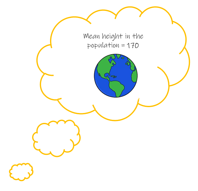
class: center, middle, inverse, title-slide .title[ # <b>Week 7: Recap</b> ] .subtitle[ ## Univariate Statistics and Methodology using R ] .author[ ### ] .institute[ ### Department of Psychology<br/>The University of Edinburgh ] --- class: inverse, center, middle # Week 1: R --- # Week 1: R  --- class: inverse, center, middle # Week 2: Distributions and Repeated Sampling --- # We collect data .pull-left[  ] .pull-right[ __Heights and Eye-Colours of USMR students__ ```r library(tidyverse) demo <- read_csv("https://uoepsy.github.io/data/surveydata_allcourse22.csv") %>% filter(course=="usmr") %>% select(height, eyecolour) %>% na.omit() dim(demo) ``` ``` ## [1] 228 2 ``` ```r head(demo) ``` ``` ## # A tibble: 6 × 2 ## height eyecolour ## <dbl> <chr> ## 1 180 brown ## 2 162 brown ## 3 175 brown ## 4 175 brown ## 5 168. brown ## 6 157. brown ``` ] --- # We can describe data .pull-left[ <!-- --> ] .pull-right[ ```r demo %>% summarise( mean_height = mean(height), sd_height = sd(height) ) ``` ``` ## # A tibble: 1 × 2 ## mean_height sd_height ## <dbl> <dbl> ## 1 168. 9.10 ``` ```r demo %>% count(eyecolour) %>% mutate(prop = n/sum(n)) ``` ``` ## # A tibble: 6 × 3 ## eyecolour n prop ## <chr> <int> <dbl> ## 1 blue 47 0.206 ## 2 brown 120 0.526 ## 3 green 26 0.114 ## 4 grey 4 0.0175 ## 5 hazel 22 0.0965 ## 6 other 9 0.0395 ``` ] --- # _what if..._ we had collected different data? .pull-left[ - Statistics we have observed from `\(n = 228\)`: - mean height: 168 - standard deviation of heights: 9.1 - proportion of people with brown eyes: 52% - Statistics that we _might have_ computed would be different. ] --- count: false # _what if..._ we had collected different data? .pull-left[ - Statistics we have observed from `\(n = 228\)`: - mean height: 168 - standard deviation of heights: 9.1 - proportion of people with brown eyes: 52% - Statistics that we _might have_ computed would be different. - Demonstration: [lecture7_demo.R](./lecture7_demo.R) ] .pull-right[ <!-- --> ] --- # quantifying sampling variation .pull-left[ __Simulations__ <!-- --> ```r mheights <- replicate(1000, mean(rnorm(n = 228, mean = 168, sd = 9.1))) sd(mheights) ``` ``` ## [1] 0.6028 ``` ] --- count: false # quantifying sampling variation (2) .pull-left[ __Simulations__ <!-- --> ```r mheights <- replicate(1000, mean(rnorm(n = 228, mean = 168, sd = 9.1))) sd(mheights) ``` ``` ## [1] 0.6028 ``` ] .pull-right[ __Maths__ sampling distribution is normally distributed with a standard deviation of: $$ `\begin{align} & \frac{\sigma}{\sqrt{n}} \\ \\ & \text{Where:} \\ & n = \text{sample size} \\ & \sigma = \text{population standard deviation} \end{align}` $$ ```r 9.1 / sqrt(228) ``` ``` ## [1] 0.6027 ``` ] --- class: inverse, center, middle # Week 3 - Test Statistics --- # What we expect vs What we observe e.g. "If the population mean height is 170, is it unlikely to see our sample's mean height of 168?" .pull-left[ __What we expect:__ <!-- --> ] -- .pull-right[ __What we observe:__ <!-- --> ] --- # Standardised Test Statistics e.g. "Given the statistics we expect, how unlikely is the statistic we observe?" .pull-left[ __Test Statistics we expect:__ <!-- --> ] .pull-right[ __Test Statistics we observe:__ <!-- --> ] --- # sampling variation in theory e.g. "Given the statistics we expect, how unlikely is the statistic we observe?" .pull-left[ __Test Statistics we expect:__ <!-- --> ] .pull-right[ <br> $$ `\begin{align} & SE = \frac{\sigma}{\sqrt{n}} \\ \\ & \text{Where:} \\ & n = \text{sample size} \\ & \sigma = \color{red}{\text{population standard deviation}} \end{align}` $$ $$ z = \frac{168 - 170}{\frac{??}{\sqrt{228}}} $$ ] --- # sampling variation in practice e.g. "Given the statistics we expect, how unlikely is the statistic we observe?" .pull-left[ __Test Statistics we expect:__ <!-- --> ] .pull-right[ <br> $$ `\begin{align} & SE = \frac{s}{\sqrt{n}} \\ \\ & \text{Where:} \\ & n = \text{sample size} \\ & s = \color{red}{\text{sample standard deviation}} \end{align}` $$ $$ t = \frac{168 - 170}{\frac{9.01}{\sqrt{228}}} $$ ] --- # statistical testing .pull-left[ 1. Assume the null hypothesis is true 2. How likely would we be to obtain our statistic in a universe where the null hypothesis is true? ] .pull-right[  ] -- ```r usmr <- read_csv("https://uoepsy.github.io/data/surveydata_allcourse22.csv") %>% filter(course=="usmr") %>% filter(!is.na(height), !is.na(eyecolour)) ``` --- # t-tests __One sample t-test__ - how far the sample mean is from some number: `$$t = \frac{\bar{x}_1 - \mu_0}{SE_{\bar{x}}}$$` ```r t.test(usmr$height, mu = 170) ``` ``` ## ## One Sample t-test ## ## data: usmr$height ## t = -3, df = 227, p-value = 0.003 ## alternative hypothesis: true mean is not equal to 170 ## 95 percent confidence interval: ## 167.0 169.4 ## sample estimates: ## mean of x ## 168.2 ``` --- # t-tests (2) __Two sample t-test__ - how far the difference in means is from zero: `$$t = \frac{\bar{x}_1 - \bar{x}_2}{SE_{\bar{x}_1-\bar{x}_2}}$$` ```r t.test(height ~ catdog, data = usmr) ``` ``` ## ## Welch Two Sample t-test ## ## data: height by catdog ## t = -1.5, df = 195, p-value = 0.1 ## alternative hypothesis: true difference in means between group cat and group dog is not equal to 0 ## 95 percent confidence interval: ## -4.2254 0.6117 ## sample estimates: ## mean in group cat mean in group dog ## 167.1 168.9 ``` --- class: inverse, center, middle # Week 4 & 5 - more test statistics --- # Chi-square tests __Chi-squared: Goodness of Fit__ $$ \chi^2 = \Sigma \frac{{(Observed-Expected)}^2}{Expected} $$ ```r table(usmr$eyecolour) ``` ``` ## ## blue brown green grey hazel other ## 47 120 26 4 22 9 ``` ```r chisq.test(table(usmr$eyecolour)) ``` ``` ## ## Chi-squared test for given probabilities ## ## data: table(usmr$eyecolour) ## X-squared = 242, df = 5, p-value <2e-16 ``` --- # Chi-square tests (2) __Chi-squared: Test of Independence__ $$ \chi^2 = \Sigma \frac{{(Observed-Expected)}^2}{Expected} $$ ```r table(usmr$ampm, usmr$catdog) ``` ``` ## ## cat dog ## Evening person 33 45 ## Morning person 18 27 ``` ```r chisq.test(table(usmr$ampm, usmr$catdog)) ``` ``` ## ## Pearson's Chi-squared test with Yates' continuity correction ## ## data: table(usmr$ampm, usmr$catdog) ## X-squared = 0.0036, df = 1, p-value = 1 ``` --- # Correlation tests __Correlation__ $$ t = \frac{r}{\sqrt{\frac{1-r^2}{n-2}}} = \frac{r}{SE_{r}} $$ ```r cor.test(usmr$sleeprating, usmr$loc) ``` ``` ## ## Pearson's product-moment correlation ## ## data: usmr$sleeprating and usmr$loc ## t = 3.4, df = 74, p-value = 0.001 ## alternative hypothesis: true correlation is not equal to 0 ## 95 percent confidence interval: ## 0.1588 0.5504 ## sample estimates: ## cor ## 0.371 ``` --- class: inverse, center, middle # and here we are!