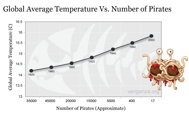
class: center, middle, inverse, title-slide # <b>Week 5: Correlations</b> ## Univariate Statistics and Methodology using R ### Martin Corley ### Department of Psychology<br/>The University of Edinburgh --- class: inverse, center, middle # Part 1: Correlation --- # Blood Alcohol and Reaction Time .pull-left[ <!-- --> - data from 100 drivers - are blood alcohol and RT systematically related? ] .pull-right[  ] ??? - the playmo crew have been out joyriding and were caught in a police speed trap - the police measured 100 people's blood alcohol and their reaction times - how would we go about telling whether two variables like this were related? --- # A Simplified Case .center[ <!-- --> ] - does `\(y\)` vary with `\(x\)`? -- - equivalent to asking "does `\(y\)` differ from its mean in the same way that `\(x\)` does?" --- count: false # A Simplified Case .center[ <!-- --> ] - does `\(y\)` vary with `\(x\)`? - equivalent to asking "does `\(y\)` differ from its mean in the same way that `\(x\)` does?" ??? here are the ways in which the values of `\(x\)` differ from `mean(x)` --- count: false # A Simplified Case .center[ <!-- --> ] - does `\(y\)` vary with `\(x\)`? - equivalent to asking "does `\(y\)` differ from its mean in the same way that `\(x\)` does?" ??? and here are the ways in which `\(y\)` varies from its mean --- # Covariance .center[ <!-- --> ] - it's likely the variables are related **if observations differ proportionately from their means** --- # Covariance ### Variance .br3.white.bg-gray.pa1[ $$ s^2 = \frac{\sum{(x-\bar{x})^2}}{n} = \frac{\sum{(x-\bar{x})(x-\bar{x})}}{n} $$ ] ??? - note that here we're using `\(n\)`, not `\(n-1\)`, because this is the whole population -- ### Covariance .br3.white.bg-gray.pa1[ $$ \textrm{cov}(x,y) = \frac{\sum{(x-\bar{x})\color{red}{(y-\bar{y})}}}{n} $$ ] ??? - note that for any (x,y), `\(x-\bar{x}\)` might be positive and `\(y-\bar{y}\)` might be positive, so the covariance could be a negative number --- # Covariance | `\(x-\bar{x}\)` | `\(y-\bar{y}\)` | `\((x-\bar{x})(y-\bar{y})\)` | |------------:|------------:|-------------------------:| | -0.3 | 1.66 | -0.5 | | 0.81 | 2.21 | 1.79 | | -1.75 | -2.85 | 4.99 | | -0.14 | -3.58 | 0.49 | | 1.37 | 2.56 | 3.52 | | | | **10.29** | .pt4[ $$ \textrm{cov}(x,y) = \frac{\sum{(x-\bar{x})(y-\bar{y})}}{n} = \frac{10.29}{5} \simeq \color{red}{2.06} $$ ] ??? - I've rounded up the numbers at the end to make this a bit neater on the slide --- # The Problem With Covariance .pull-left[ **Miles** | `\(x-\bar{x}\)` | `\(y-\bar{y}\)` | `\((x-\bar{x})(y-\bar{y})\)` | |------------:|------------:|-------------------------:| | -0.3 | 1.66 | -0.5 | | 0.81 | 2.21 | 1.79 | | -1.75 | -2.85 | 4.99 | | -0.14 | -3.58 | 0.49 | | 1.37 | 2.56 | 3.52 | | | | **10.29** | $$ \textrm{cov}(x,y)=\frac{10.29}{5}\simeq 2.06 $$ ] .pull-right[ **Kilometres** | `\(x-\bar{x}\)` | `\(y-\bar{y}\)` | `\((x-\bar{x})(y-\bar{y})\)` | |------------:|------------:|-------------------------:| | -0.48 | 2.68 | -1.29 | | 1.3 | 3.56 | 4.64 | | -2.81 | -4.59 | 12.91 | | -0.22 | -5.77 | 1.27 | | 2.21 | 4.12 | 9.12 | | | | **26.65** | $$ \textrm{cov}(x,y)=\frac{26.65}{5}\simeq 5.33 $$ ] ??? - these are exactly the same 'values' so they should each be as correlated as the other - so we need to divide covariance by something to represent the overall "scale" of the units --- # Correlation Coefficient - the standardised version of covariance is the **correlation coefficient**, `\(r\)` $$ r = \frac{\textrm{covariance}(x,y)}{\textrm{standard deviation}(x)\cdot\textrm{standard deviation}(y)} $$ -- .pt3[ $$ r=\frac{\frac{\sum{(x-\bar{x})(y-\bar{y})}}{\color{red}{N}}}{\sqrt{\frac{\sum{(x-\bar{x})^2}}{\color{red}{N}}}\sqrt{\frac{\sum{(y-\bar{y})^2}}{\color{red}{N}}}} $$ ] -- .pt1[ $$ r=\frac{\sum{(x-\bar{x})(y-\bar{y})}}{\sqrt{\sum{(x-\bar{x})^2}}\sqrt{\sum{(y-\bar{y})^2}}} $$ ] --- # Correlation Coefficient - measure of _how related_ two variables are - `\(-1 \le r \le 1\)` ( `\(\pm 1\)` = perfect fit; `\(0\)` = no fit; sign shows direction of slope ) .pull-left[  $$ r=0.4648 $$ ] .pull-right[ <!-- --> $$ r=-0.4648 $$ ] ??? - on the left, we have the drunken drivers from our first slide, and you can see that there is a moderate positive correlation + the higher your blood alcohol, the slower your RT - on the right, we have a negative correlation: what the drivers _think_ happens + the higher your blood alcohol, the _faster_ your RT --- # What Does the Value of _r_ Mean? <!-- --> --- class: inverse, center, middle, animated, bounceInUp # Intermission --- class: inverse, center, middle # Part 1a ## Correlations Contd. --- # Significance of a Correlation .pull-left[  $$ r = 0.4648 $$ ] .pull-right[  ] ??? - the police have stopped our friends and measured their blood alcohol - is their evidence sufficient to conclude that there is likely to be a relationship between blood alcohol and reaction time? --- # Significance of a Correlation - we can measure a correlation using `\(r\)` - we want to know whether that correlation is **significant** + i.e., whether the probability of finding it by chance is low enough .pt2[ - cardinal rule in NHST: compare everything to chance - let's investigate... ] --- # Random Correlations - function to pick some pairs of numbers entirely at random, return correlation - arbitrarily, I've picked numbers uniformly distributed between 0 and 100 ```r x <- runif(5, min=0, max=100) y <- runif(5, min=0, max=100) cbind(x,y) ``` ``` ## x y ## [1,] 58.38 82.33 ## [2,] 77.90 17.03 ## [3,] 56.58 21.52 ## [4,] 47.06 27.70 ## [5,] 73.68 29.14 ``` ```r cor(x,y) ``` ``` ## [1] -0.254 ``` --- count: false # Random Correlations - function to pick some pairs of numbers entirely at random, return correlation - arbitrarily, I've picked numbers uniformly distributed between 0 and 100 .flex.items-top[ .w-50.pa2[ ```r randomCor <- function(size) { x <- runif(size, min=0, max=100) y <- runif(size, min=0, max=100) cor(x,y) # calculate r } # then we can use the usual trick: rs <- replicate(1000, randomCor(5)) hist(rs) ``` ] .w-50.pa2[  ]] --- # Random Correlations .pull-left[ <!-- --> ] .pull-right[ <!-- --> ] --- # Larger Sample Size .pull-left[ <!-- --> ] .pull-right[ - distribution of random `\(r\)`s is `\(t\)` distribution, with `\(n-2\)` df $$ t= r\sqrt{\frac{n-2}{1-r^2}} $$ - makes it "easy" to calculate probability of getting `\(\ge{}r\)` for sample size `\(n\)` by chance ] --- # Pirates and Global Warming .center[  ] - clear _negative_ correlation between number of pirates and mean global temperature - we need pirates to combat global warming --- # Simpson's Paradox .center[ <!-- --> ] - the more hours of exercise, the greater the risk of disease --- # Simpson's Paradox .center[ <!-- --> ] - age groups mixed together - an example of a _mediating variable_ --- # Interpreting Correlation - correlation does not imply causation - correlation simply suggests that two variables are related + there may be mediating variables - interpretation of that relationship is key - never rely on statistics such as `\(r\)` without + looking at your data + thinking about the real world --- class: inverse, center, middle, animated, bounceInUp # End of Part 1 --- class: inverse, center, middle # Part 2 --- # Has Statistics Got You Frazzled? .pull-left[  ] .pull-right[ - we've bandied a lot of terms around in quite a short time - we've tended to introduce them by example - time to step back... ] --- class: inverse, center, middle # Part Z: The Zen of Stats .center[  ] --- # What is NHST all about? ## **N**ull **H**ypothesis **S**tatistical **T**esting - two premises 1. much of the variation in the universe is due to _chance_ 1. we can't _prove_ a hypothesis that something else is the cause --- # Chance .pull-left[ - when we say _chance_, what we really mean is "stuff we didn't measure" - we believe that "pure" chance conforms approximately to predictable patterns (like the normal and `\(t\)` distributions) - if our data isn't in a predicted pattern, perhaps we haven't captured all of the non-chance elements ] .pull-right[ ### pattens attributable to <!-- --> ] ??? - we'll come back to looking at the patterns later on; essentially there is always going to be some part of any variation we can't explain --- # Proof .pull-left[  ] .pull-right[ - can't prove a hypothesis to be true - "the sun will rise tomorrow" ] --- count: false # Proof .pull-left[  ] .pull-right[ - can't prove a hypothesis to be true - "the sun will rise tomorrow" - _just takes one counterexample_ ] --- # Chance and Proof .br3.pa2.bg-gray.white[if the likelihood that the pattern of data we've observed would be found _by chance_ is low enough, propose an alternative explanation ] - work from summaries of the data (e.g., `\(\bar{x}\)`, `\(\sigma\)`) - use these to approximate chance (e.g., `\(t\)` distribution) -- + catch: we can't estimate the probability of an exact value (this is an example of the measurement problem) + estimate the probability of finding the measured difference _or more_ --- # Alpha and Beta - we need an agreed "standard" for proposing an alternative explanation + typically in psychology, we set `\(\alpha\)` to 0.05 + "if the probability of finding this difference or more under chance is `\(\alpha\)` (e.g., 5%) or less, propose an alternative" - we also need to understand the quality of evidence we're providing + can be measured using `\(\beta\)` (psychologists typically aim for 0.80) + "given that an effect truly exists in a population, what is the probability of finding `\(p<\alpha\)` in a sample (of size `\(n\)` etc.)?" --- class: middle background-image: url(lecture_5_files/img/nuts-and-bolts.jpg) .br3.pa2.bg-white-80[ # The Rest is Just Nuts and Bolts - type of measurement - relevant laws of chance - suitable estimated distribution (normal, `\(t\)`, `\(\chi^2\)`, etc.) - suitable summary statistic ( `\(z\)`, `\(t\)`, `\(\chi^2\)`, `\(r\)`, etc.) - use statistic and distribution to calculate `\(p\)` and compare to `\(\alpha\)` - rinse, repeat ] --- # The Most Useful Tool .pull-left[  ] .pull-right[ - `\(t\)` (or `\(z\)`) statistics are really ubiquitous - formally, mean difference divided by standard error - conceptually: + what is the difference? + what is the range of differences I would get by chance? + how extreme is this difference compared to the range? - expressed in terms of _numbers of standard errors_ from the most likely difference (usually, by hypothesis, zero) ] --- class: inverse, center, middle # Part N: Nirvana .center[  ] --- # .red[Announcement] .flex.items-center[ .w-50.pa2[ - no lecture or lab released in week 6 (25-29 October) - quiz 2 due on Friday 29th - after the break: linear models - in the meantime, have a good break and a Happy Halloween ] .w-50.pa2[  ]] --- class: inverse, center, middle, animated, bounceInUp # End --- # Acknowledgements - the [papaja package](https://github.com/crsh/papaja) helps with the preparation of APA-ready manuscripts - icons by Diego Lavecchia from the [Noun Project](https://thenounproject.com/)