
Introduction to the Linear Model
DPUK Spring Academy
2025-04-01
The Linear Model
Our model \(\hat{\textrm{f}}\textrm{itted}\) to some data:
\(\hat{y}_i = \color{blue}{\hat b_0 \cdot{} 1 + \hat b_1 \cdot{} x_i}\)
For the \(i^{th}\) observation:
- \(\color{red}{y_i}\) is the value we observe for \(x_i\)
- \(\hat{y}_i\) is the value the model predicts for \(x_i\)
- \(\color{red}{y_i} = \hat{y}_i + \hat\varepsilon_i\)

An example
Our model \(\hat{\textrm{f}}\textrm{itted}\) to some data:
\(\color{red}{y_i} = \color{blue}{5 \cdot{} 1 + 2 \cdot{} x_i} + \hat\varepsilon_i\)
For the observation \(x_i = 1.2, \; y_i = 9.9\):
\[ \begin{align} \color{red}{9.9} & = \color{blue}{5 \cdot{}} 1 + \color{blue}{2 \cdot{}} 1.2 + \hat\varepsilon_i \\ & = 7.4 + \hat\varepsilon_i \\ & = 7.4 + 2.5 \\ \end{align} \]

Categorical Predictors
| y | x |
|---|---|
| 7.99 | Category1 |
| 4.73 | Category0 |
| 3.66 | Category0 |
| 3.41 | Category0 |
| 5.75 | Category1 |
| 5.66 | Category0 |
| ... | ... |

Null Hypothesis Testing

Null Hypothesis Testing

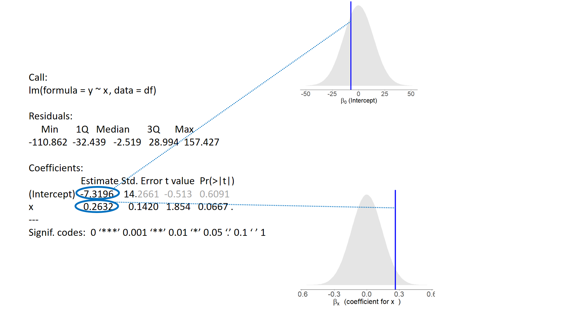
test of individual parameters
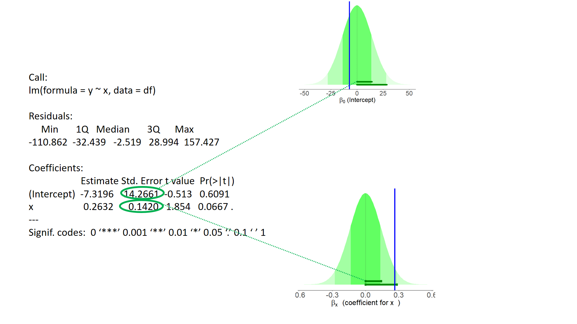
test of individual parameters (2)
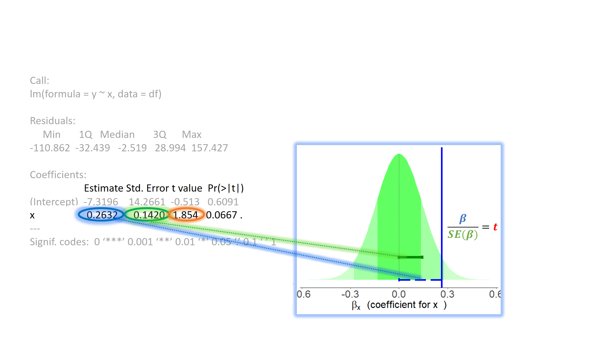
test of individual parameters (3)
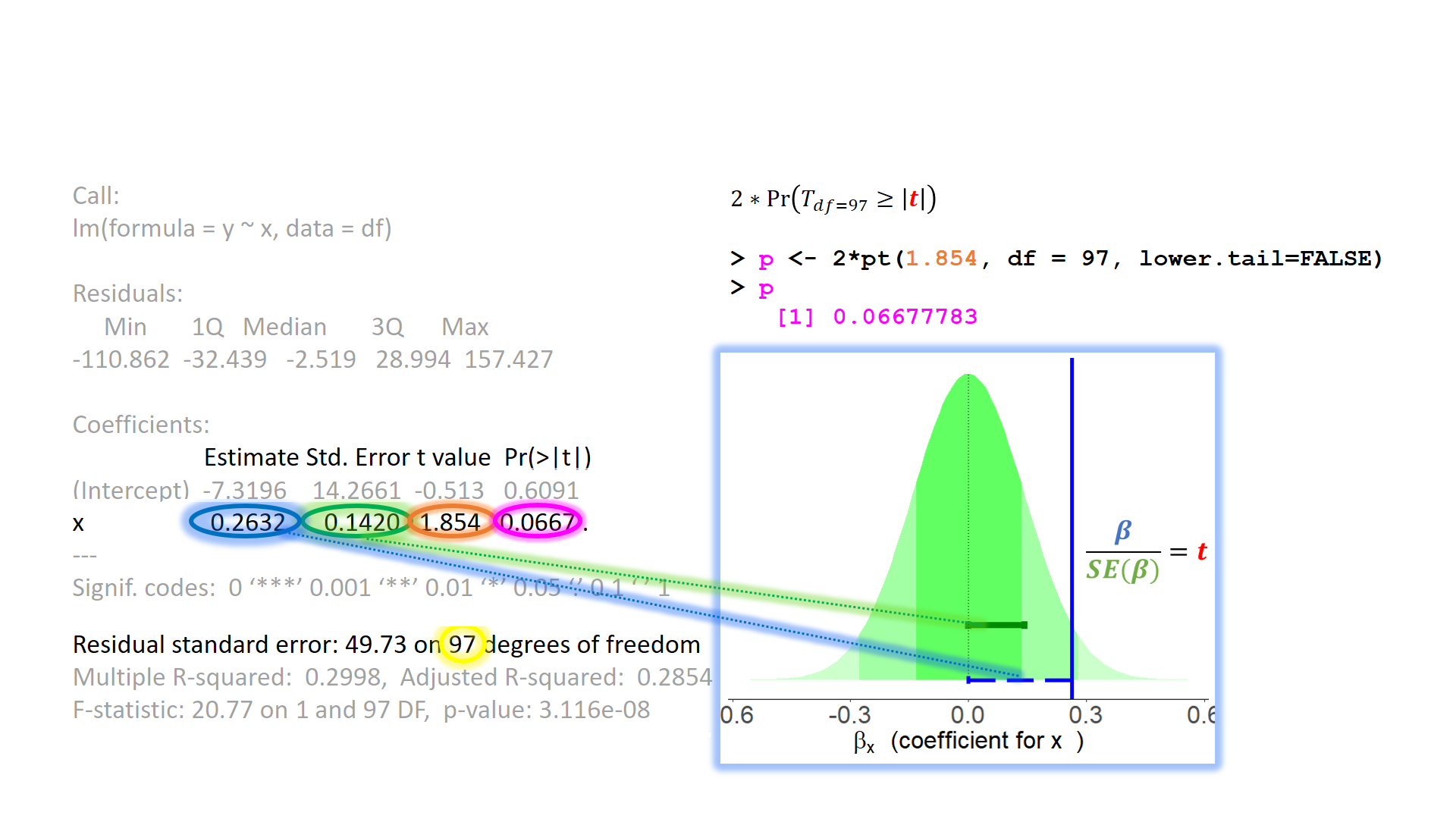
test of individual parameters (4)
Sums of Squares
Rather than focussing on slope coefficients, we can also think of our model in terms of sums of squares (SS).
\(SS_{total} = \sum^{n}_{i=1}(y_i - \bar y)^2\)
\(SS_{model} = \sum^{n}_{i=1}(\hat y_i - \bar y)^2\)
\(SS_{residual} = \sum^{n}_{i=1}(y_i - \hat y_i)^2\)

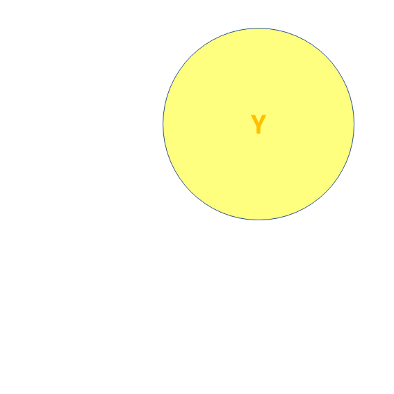
![]() Third variables
Third variables
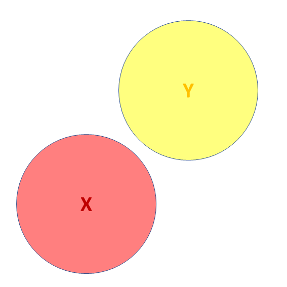
![]() Third variables
Third variables
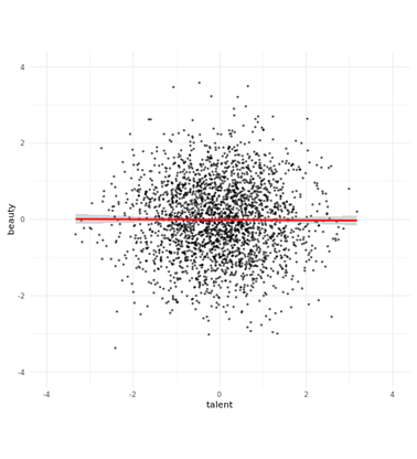
- X and Y are ‘orthogonal’ (perfectly uncorrelated)
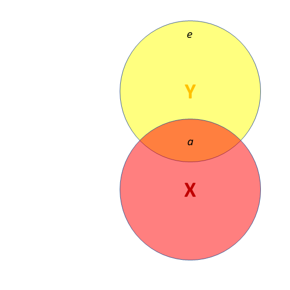
![]() Third variables
Third variables
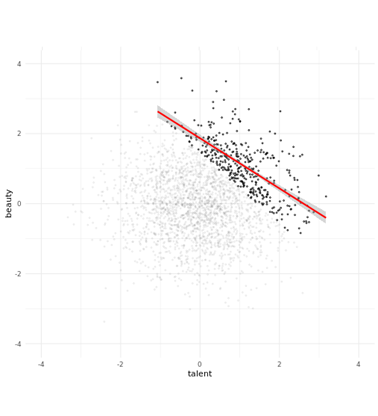
- X and Y are correlated.
- a = portion of Y’s variance shared with X
- e = portion of Y’s variance unrelated to X
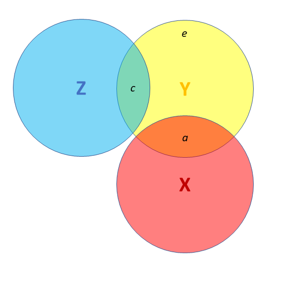
![]() Third variables
Third variables
- X and Y are correlated.
- a = portion of Y’s variance shared with X
- e = portion of Y’s variance unrelated to X
- Z is also related to Y (c)
- Z is orthogonal to X (no overlap)
- relation between X and Y is unaffected (a)
- unexplained variance in Y (e) is reduced, so a:e ratio is greater.
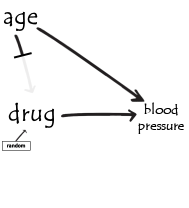
Design is so important! If possible, we could design it so that X and Z are orthogonal (in the long run) by e.g., randomisation.
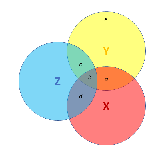
![]() Third variables
Third variables
- X and Y are correlated.
- Z is also related to Y (c + b)
- Z is related to X (b + d)
Association between X and Y is changed if we adjust for Z (a is smaller than previous slide), because there is a bit (b) that could be attributed to Z instead.
- multiple regression coefficients for X and Z are like areas a and c (scaled to be in terms of ‘per unit change in the predictor’)
- total variance explained by both X and Z is a+b+c
I have control issues..
..and so should you
what do we mean by “control”?
- often quite a vague/nebulous idea
relationship between x and y …
- controlling for z
- accounting for z
- conditional upon z
- holding constant z
- adjusting for z
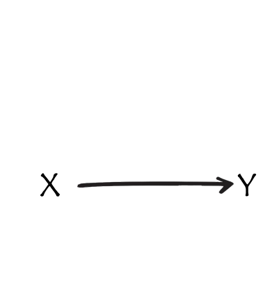
thus far - lm(y~x)
what do i do?
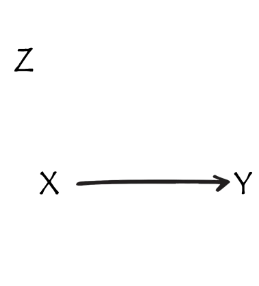
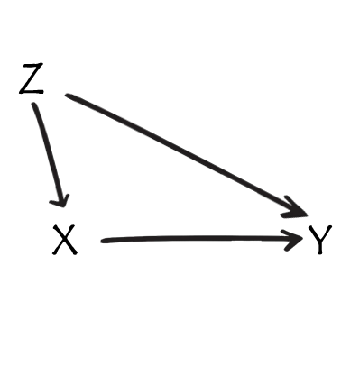
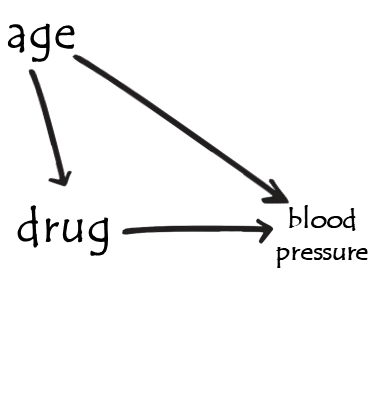
Z is a confounder
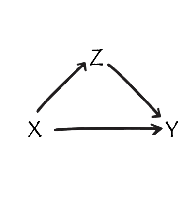
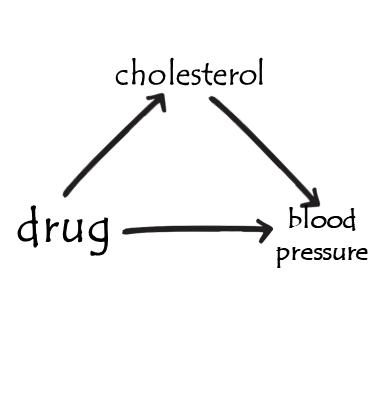
Z is a mediator
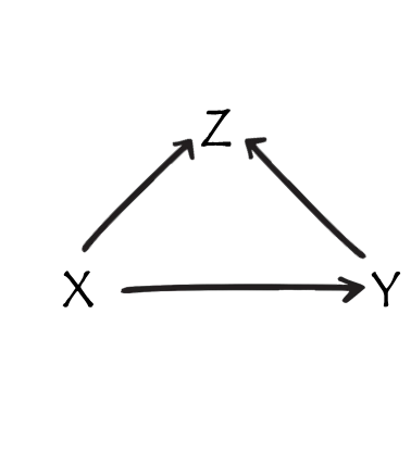
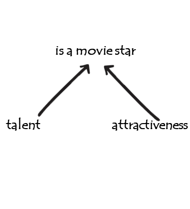
Z is a collider
example
example
example
example
example 2
- to play around with this, see https://colliderbias.herokuapp.com/
example 2
- to play around with this, see https://colliderbias.herokuapp.com/
example 2
- to play around with this, see https://colliderbias.herokuapp.com/
More than one predictor?
\(\color{red}{y} = \color{blue}{b_0 \cdot{} 1 + b_1 \cdot{} x_1 + \, ... \, + b_k \cdot x_k} + \varepsilon\)
mymodel <- lm(y ~ 1 + x1 + ... + xk, data = mydata)
tests of multiple parameters
Model comparisons:
m1 <- lm(y ~ 1 + x, data = df)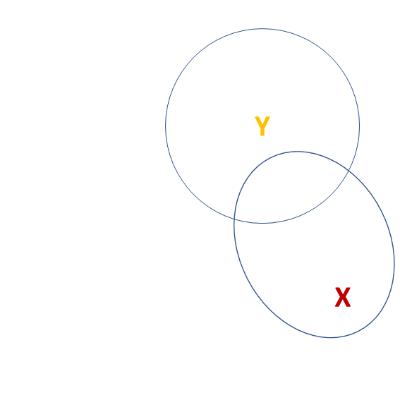
m2 <- lm(y ~ 1 + z + z2 + x, data = df)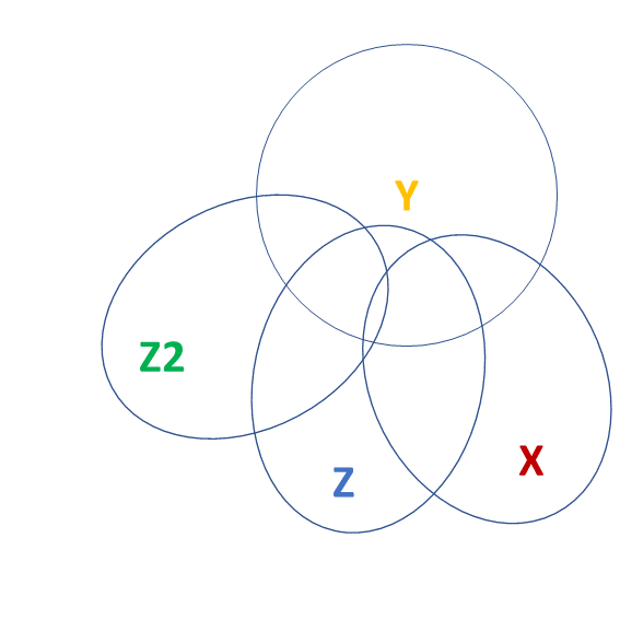
tests of multiple parameters (2)
isolate the improvement in model fit due to inclusion of additional parameters
m1 <- lm(y ~ 1 + x, data = df)
m2 <- lm(y ~ 1 + z + z2 + x, data = df)
anova(m1, m2)
Analysis of Variance Table
Model 1: y ~ 1 + x
Model 2: y ~ 1 + z + z2 + x
Res.Df RSS Df Sum of Sq F Pr(>F)
1 98 1141
2 96 357 2 785 106 <2e-16 ***
---
Signif. codes: 0 '***' 0.001 '**' 0.01 '*' 0.05 '.' 0.1 ' ' 1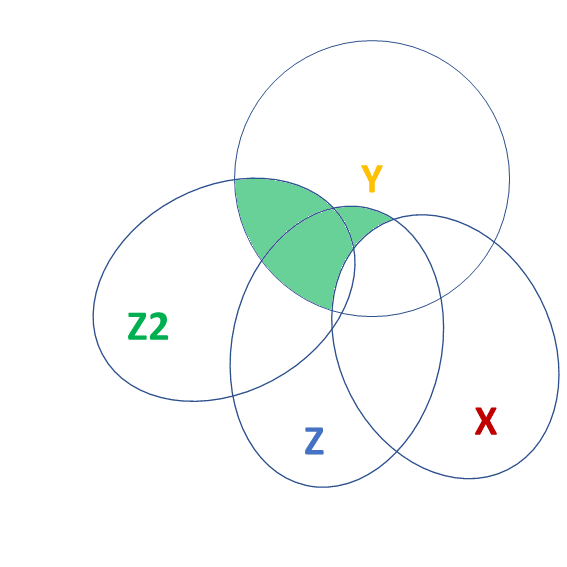
tests of multiple parameters (3)
Test everything in the model all at once by comparing it to a ‘null model’ with no predictors:
m0 <- lm(y ~ 1, data = df)
m2 <- lm(y ~ 1 + z2 + z + x, data = df)

anova(m0, m2)
Analysis of Variance Table
Model 1: y ~ 1
Model 2: y ~ 1 + z2 + z + x
Res.Df RSS Df Sum of Sq F Pr(>F)
1 99 1232
2 96 357 3 875 78.6 <2e-16 ***
---
Signif. codes: 0 '***' 0.001 '**' 0.01 '*' 0.05 '.' 0.1 ' ' 1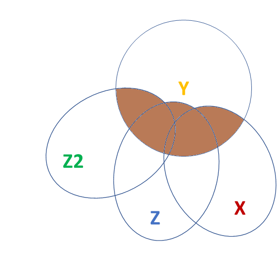
multiple regression model
\(\color{red}{y} = \color{blue}{b_0 \cdot{} 1 + b_1 \cdot{} x_1 + \, ... \, + b_k \cdot x_k} + \varepsilon\)
mymodel <- lm(y ~ 1 + x1 + ... + xk, data = mydata)
Think in hypotheticals
mod = lm(stress ~ age, data = df)
summary(mod)
Coefficients:
Estimate Std. Error t value Pr(>|t|)
(Intercept) -3.8755 2.3911 -1.62 0.1437
age 0.2187 0.0633 3.46 0.0086 **
---
Signif. codes: 0 '***' 0.001 '**' 0.01 '*' 0.05 '.' 0.1 ' ' 1
Residual standard error: 3.08 on 8 degrees of freedom
Multiple R-squared: 0.599, Adjusted R-squared: 0.549
F-statistic: 11.9 on 1 and 8 DF, p-value: 0.00862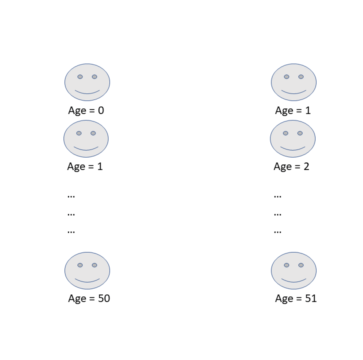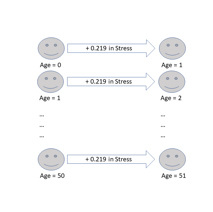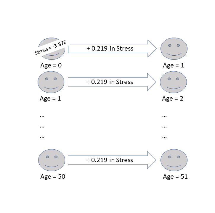
Think in hypotheticals
mod = lm(stress ~ therapy, data = df)
summary(mod)
Coefficients:
Estimate Std. Error t value Pr(>|t|)
(Intercept) 5.45 1.99 2.75 0.025 *
therapy -3.57 2.81 -1.27 0.240
---
Signif. codes: 0 '***' 0.001 '**' 0.01 '*' 0.05 '.' 0.1 ' ' 1
Residual standard error: 4.44 on 8 degrees of freedom
Multiple R-squared: 0.168, Adjusted R-squared: 0.0637
F-statistic: 1.61 on 1 and 8 DF, p-value: 0.24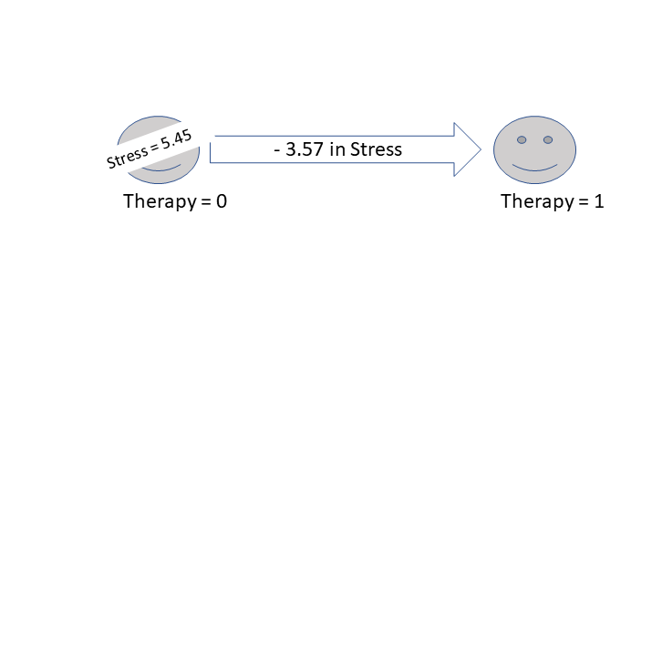
Think in hypotheticals
mod = lm(stress ~ age + exercise + therapy, data = df)
summary(mod)
Coefficients:
Estimate Std. Error t value Pr(>|t|)
(Intercept) 3.0874 3.1338 0.99 0.36259
age 0.2412 0.0334 7.22 0.00036 ***
exercise -0.9082 0.4817 -1.89 0.10836
therapy -6.9398 1.6246 -4.27 0.00525 **
---
Signif. codes: 0 '***' 0.001 '**' 0.01 '*' 0.05 '.' 0.1 ' ' 1
Residual standard error: 1.61 on 6 degrees of freedom
Multiple R-squared: 0.918, Adjusted R-squared: 0.877
F-statistic: 22.3 on 3 and 6 DF, p-value: 0.00118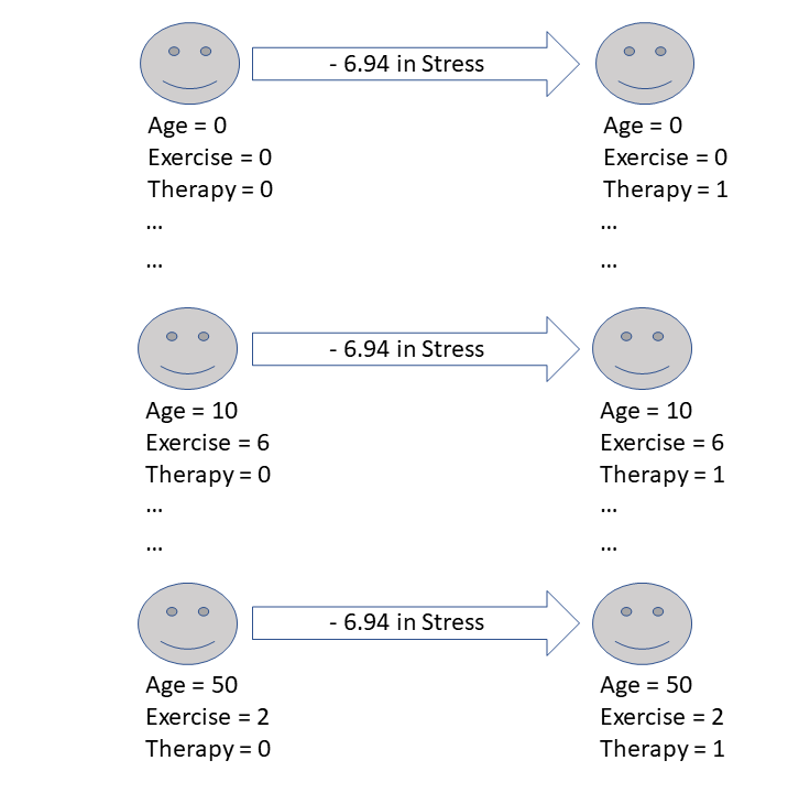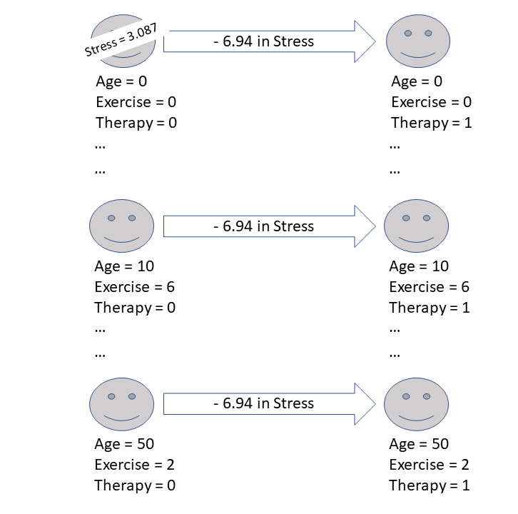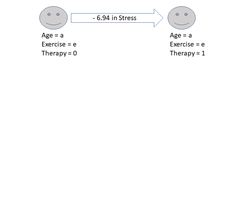
example - simple regression
head(braindata)# A tibble: 6 × 4
species mass_brain age isMonkey
<chr> <dbl> <dbl> <chr>
1 Rhesus monkey 0.449 5 YES
2 Human 0.577 2 NO
3 Potar monkey 0.349 30 YES
4 Human 0.626 27 NO
5 Potar monkey 0.316 31 YES
6 Rhesus monkey 0.398 11 YES 
example - in multiple regression
head(braindata)# A tibble: 6 × 4
species mass_brain age isMonkey
<chr> <dbl> <dbl> <chr>
1 Rhesus monkey 0.449 5 YES
2 Human 0.577 2 NO
3 Potar monkey 0.349 30 YES
4 Human 0.626 27 NO
5 Potar monkey 0.316 31 YES
6 Rhesus monkey 0.398 11 YES 
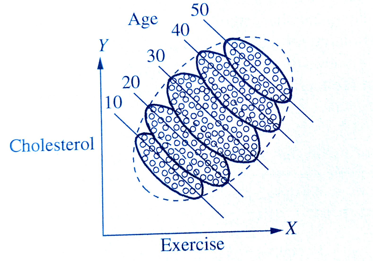
example - multiple levels
more levels = more dimensions

example - multiple levels
lm(mass_brain ~ species, data = braindata) |>
  summary()
Call:
lm(formula = mass_brain ~ species, data = braindata)

Residuals:
     Min       1Q   Median       3Q      Max
-0.30010 -0.06254  0.00129  0.04779  0.18664

Coefficients:
                     Estimate Std. Error t value Pr(>|t|)
(Intercept)            0.6027     0.0275   21.94  < 2e-16 ***
speciesPotar monkey   -0.3574     0.0414   -8.63  7.4e-10 ***
speciesRhesus monkey  -0.1526     0.0426   -3.59   0.0011 **
---
Signif. codes:  0 '***' 0.001 '**' 0.01 '*' 0.05 '.' 0.1 ' ' 1

Residual standard error: 0.103 on 32 degrees of freedom
Multiple R-squared:  0.699, Adjusted R-squared:  0.681
F-statistic: 37.2 on 2 and 32 DF,  p-value: 4.45e-09