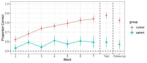
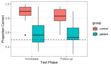
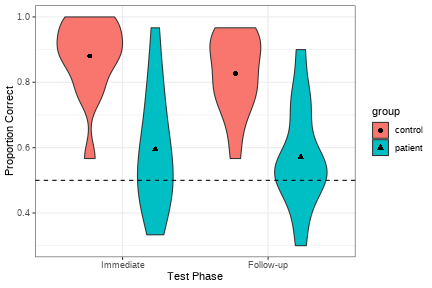
class: center, middle, inverse, title-slide # <b>Week 2: Logistic Multilevel Modeling</b> ## Multivariate Statistics and Methodology using R (MSMR)<br><br> ### Dan Mirman ### Department of Psychology<br>The University of Edinburgh --- # Why logistic regression? (A brief review) Aggregated binary outcomes (e.g., accuracy, fixation proportion) can look approximately continuous, but they * Are bounded: can only have values between 0.0 and 1.0 * Have very specific, non-uniform variance pattern <img src="./figs/BinomVariance.png" width="35%" /> --- # Why logistic regression? (A brief review) These properties can produce incorrect results in linear regression. <img src="./figs/LinLogDemoBoxplotTables.png" width="90%" /> --- # Logistic regression (A brief review) * Model the binomial process that produced binary data * Not enough to know that accuracy was 90%, need to know whether that was 9 out of 10 trials or 90 out of 100 trials * Can be a binary vector of single-trial 0's (failures, No's) or 1's (successes, Yes's) * More compact version: count of the number of successes and the number of failures Outcome is log-odds (also called "logit"): `\(logit(Yes, No) = \log \left(\frac{Yes}{No}\right)\)` Compare to proportions: `\(p(Yes, No) = \frac{Yes}{Yes+No}\)` Note: logit is undefined (`Inf`) when `\(p=0\)` or `\(p=1\)`, this makes it hard to fit logistic models to data with such extreme values (e.g., fixations on objects that are very rarely fixated). --- # Example Data Novel word learning (`nwl`) in aphasia (based on Peñaloza et al., 2016). Participants were 27 older adults (13 with aphasia, 14 control) who completed a short training session to learn 6 new words: made-up labels for ancient farming equipment. There were 7 blocks of training trials, followed by an immediate recall test block, and there was a follow-up test block 1 week later. Each block consisted of 30 2AFC trials, feedback was provided during the training blocks but not during the test blocks. ```r load("./data/nwl.RData") summary(nwl) ``` ``` ## group lesion_location block PropCorrect NumCorrect ## control:126 anterior : 45 Min. :1 Min. :0.200 Min. : 6.0 ## patient:117 posterior: 63 1st Qu.:3 1st Qu.:0.533 1st Qu.:16.0 ## NA's :135 Median :5 Median :0.700 Median :21.0 ## Mean :5 Mean :0.682 Mean :20.5 ## 3rd Qu.:7 3rd Qu.:0.833 3rd Qu.:25.0 ## Max. :9 Max. :1.000 Max. :30.0 ## ## NumError ID Phase ## Min. : 0.00 control1 : 9 Length:243 ## 1st Qu.: 5.00 control10: 9 Class :character ## Median : 9.00 control11: 9 Mode :character ## Mean : 9.54 control12: 9 ## 3rd Qu.:14.00 control13: 9 ## Max. :24.00 control14: 9 ## (Other) :189 ``` --- # Example Data ```r ggplot(nwl, aes(block, PropCorrect, color=group, shape=group)) + stat_summary(fun.data=mean_se, geom="pointrange") + stat_summary(data=filter(nwl, block <= 7), fun=mean, geom="line") + geom_hline(yintercept=0.5, linetype="dashed") + geom_vline(xintercept=c(7.5, 8.5), linetype="dashed") + scale_x_continuous(breaks=1:9, labels=c(1:7, "Test", "Follow-Up")) + expand_limits(y=1.0) + theme_bw() + labs(x="Block", y="Proportion Correct") ``` <!-- --> --- # Research questions (just focus on test data for now) .pull-left[ <!-- --> ] .pull-right[ * Were patients with aphasia less successful than controls were at learning these new words? (Lower test performance) * Did recall decrease from immediate test to 1-week follow-up? * Was retention (recall decrease) different for the two groups? ] -- One might be tempted to test this with a 2x2 ANOVA. In what ways is that right? In what ways is that wrong? -- * What it gets right + Group as a between-participant variable, Phase as a within-participant variable (MLM is a more flexible version of repeated measures ANOVA) + Phase-by-group interaction -- * What it gets wrong: Accuracy is not a continuous linear variable, it is an aggregated binary variable --- # Logistic MLM: Fit the model Logistic model code is almost the same as linear model code. Three differences: 1. `glmer()` instead of `lmer()` 2. outcome is 1/0 or aggregated number of 1s, 0s 3. add `family=binomial` ```r m.recall <- glmer(cbind(NumCorrect, NumError) ~ Phase * group + (Phase | ID), data=filter(nwl, block > 7), family="binomial") ``` ``` ## boundary (singular) fit: see ?isSingular ``` -- Note: Logistic MLMs are slower to fit and are prone to convergence problems. * May need to simplify random effect structure * Convergence warnings: A warning is not an error -- will need to check parameter estimates and SE * Singular fit message: A message is not an error -- will need to assess reason for message and consider changes to the model --- # Logistic MLM: Model summary .scroll-output[ ```r summary(m.recall) ``` ``` ## Generalized linear mixed model fit by maximum likelihood (Laplace ## Approximation) [glmerMod] ## Family: binomial ( logit ) ## Formula: cbind(NumCorrect, NumError) ~ Phase * group + (Phase | ID) ## Data: filter(nwl, block > 7) ## ## AIC BIC logLik deviance df.resid ## 283.2 297.1 -134.6 269.2 47 ## ## Scaled residuals: ## Min 1Q Median 3Q Max ## -1.2676 -0.4586 0.0526 0.4553 1.2636 ## ## Random effects: ## Groups Name Variance Std.Dev. Corr ## ID (Intercept) 0.4635 0.681 ## PhaseImmediate 0.0505 0.225 1.00 ## Number of obs: 54, groups: ID, 27 ## ## Fixed effects: ## Estimate Std. Error z value Pr(>|z|) ## (Intercept) 1.719 0.231 7.45 9.1e-14 *** ## PhaseImmediate 0.582 0.232 2.51 0.012 * ## grouppatient -1.388 0.316 -4.40 1.1e-05 *** ## PhaseImmediate:grouppatient -0.441 0.278 -1.59 0.113 ## --- ## Signif. codes: 0 '***' 0.001 '**' 0.01 '*' 0.05 '.' 0.1 ' ' 1 ## ## Correlation of Fixed Effects: ## (Intr) PhsImm grpptn ## PhaseImmedt -0.141 ## grouppatint -0.725 0.094 ## PhsImmdt:gr 0.108 -0.800 -0.066 ## optimizer (Nelder_Mead) convergence code: 0 (OK) ## boundary (singular) fit: see ?isSingular ``` ] --- # Contrast coding In `R`, the default for factors is "treatment" coding: the reference level is the baseline. This means that the parameter estimates are *simple* effects. * `PhaseImmediate`: effect of test phase *for control group* (reference level of `group`) * `grouppatient`: effect of group *at follow-up* (reference level for `Phase`) -- ### To estimate main effects, need to use "sum" coding ```r m.recall_sum <- glmer(cbind(NumCorrect, NumError) ~ Phase * group + (Phase | ID), contrasts = list(Phase = "contr.sum", group = "contr.sum"), data=filter(nwl, block > 7), family="binomial") coef(summary(m.recall_sum)) ``` ``` ## Estimate Std. Error z value Pr(>|z|) ## (Intercept) 1.2060 0.16911 7.132 9.917e-13 ## Phase1 -0.1808 0.07326 -2.468 1.359e-02 ## group1 0.8045 0.16819 4.783 1.725e-06 ## Phase1:group1 -0.1102 0.06946 -1.587 1.125e-01 ``` --- # Logistic MLM: Plot model fit The `fitted` function conveniently returns proportions from a logistic model, so plotting the model fit is easy: ```r ggplot(filter(nwl, block > 7), aes(fct_rev(Phase), PropCorrect, fill=group)) + geom_violin() + stat_summary(aes(y=fitted(m.recall_sum), shape=group), fun=mean, geom = "point", size=2, position=position_dodge(width=.9)) + geom_hline(yintercept = 0.5, linetype="dashed") + theme_bw() + labs(y="Proportion Correct", x="Test Phase") ``` <!-- --> --- # Simplify random effects There is some disagreement about the *right* way to structure random effects. The core issues are: 1. For within-subject variables, omitting the random effect tends to inflate false positive rates of the corresponding fixed effect (Barr et al., 2013). So if you want to make inferences about a (within-subject) fixed effect, you should include the corresponding random effect (*Keep it maximal*). -- 2. Random effects require a lot of data to estimate, so it is easy to over-parameterize a model with random effects (you'll get convergence warnings or messages). Poor convergence can mean that there may be other fixed effect estimates that are (nearly) equally good at describing your data, which is a problem since you want to make inferences based on the fixed effect estimates. -- ### Solutions * Start with a maximal random effect structure * In case of convergence problems, look at the random effect variance-covariance matrix: are there terms with very low variance or unrealistic covariance (-1 or 1)? Consider removing these. * Compare fixed effect estimates under different random effect structures: ideally, the fixed effect estimates and SE should be (approximately) the same. If they are substantially different, then your modeling approach is not robust and you should reconsider and/or be *very* cautious about interpreting the results.