class: center, middle, inverse, title-slide # <b>Week 1: Introduction to Multilevel Modeling</b> ## Multivariate Statistics and Methodology using R (MSMR)<br><br> ### Dan Mirman ### Department of Psychology<br>The University of Edinburgh --- # What are nested data? Data that have hierarchical or clustered structure * Clustered observations (ex: multiple children in one family or classroom or neighborhood) * Repeated measures (ex: multiple questions on an exam, any within-subject manipulation) * Longitudinal data (ex: height of children) -- **Very common in psychological science** --- # Gradual change (based on a true story) 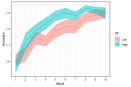<!-- --> -- * Novel word learning is faster for high TP than low TP words -- * But, t-test on overall mean accuracy is marginal (p=0.096) -- * Repeated measures ANOVA shows main effect of Block, marginal effect of TP, and no interaction (F<1) -- * Block-by-block t-test significant only in block 4 and marginal in block 5 --- # Two key features ### Nested data are not independent * A child that is taller-than-average at time *t*, is likely to be taller-than-average at time *t+1* * Non-independence is related to individual differences * Nesting can happen on multiple levels: children within families or hospitals -- ### Can be related by continuous variable (i.e., time, but could be [letter] size, number of distractors, etc.) * Ought to model this variable as continuous * Can quantify trajectories/shapes of change --- # Why use multilevel models for nested data? * Correctly model non-independence of observations * Estimate group-level and individual-level effects (same for other levels) * Model trajectories of change -- ### Nomenclature note All of these terms refer to the same family of statistical methods, with slight differences in term preference across application domains and in implied data type: * Multilevel models (MLM), Multilevel regression (MLR) * Hierarchical linear modeling (HLM) * Mixed effects models (MEM), Mixed effects regression (MER), Linear mixed models (LMM) * Growth curve analysis (GCA; implies longitudinal data with non-linear change) --- # Linear regression: A brief review 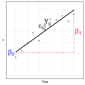<!-- --> -- `\(Y = \beta_{0} + \beta_{1} \cdot Time\)` -- `\(Y_{ij} = \beta_{0i} + \beta_{1i} \cdot Time_{j} + \epsilon_{ij}\)` -- __Fixed effects__: <span style="color:blue"> `\(\beta_{0}\)` </span> (Intercept), <span style="color:red"> `\(\beta_{1}\)` </span> (Slope) -- __Random effects__: `\(\epsilon_{ij}\)` (Residual error) --- # Multilevel models: Fixed effects Level 1: `\(Y_{ij} = \beta_{0i} + \beta_{1i} \cdot Time_{j} + \epsilon_{ij}\)` -- Level 2: model of the Level 1 parameter(s) `\(\beta_{0i} = \gamma_{00} + \zeta_{0i}\)` * `\(\gamma_{00}\)` is the population mean * `\(\zeta_{0i}\)` is individual deviation from the mean -- `\(\beta_{0i} = \gamma_{00} + \gamma_{0C} \cdot C + \zeta_{0i}\)` * `\(\gamma_{0C}\)` is the fixed effect of condition `\(C\)` on the *intercept* -- `\(\beta_{1i} = \gamma_{10} + \gamma_{1C} \cdot C + \zeta_{1i}\)` * `\(\gamma_{1C}\)` is the fixed effect of condition `\(C\)` on the *slope* --- # Multilevel models: Random effects Level 1: `\(Y_{ij} = \beta_{0i} + \beta_{1i} \cdot Time_{j} + \epsilon_{ij}\)` Level 2: `\(\beta_{0i} = \gamma_{00} + \gamma_{0C} \cdot C + \zeta_{0i}\)` `\(\beta_{1i} = \gamma_{10} + \gamma_{1C} \cdot C + \zeta_{1i}\)` Residual errors * `\(\zeta_{0i}\)` unexplained variance in *intercept* * `\(\zeta_{1i}\)` unexplained variance in *slope* * Unexplained variance reflects individual differences * Random effects require a lot of data to estimate --- # Fixed vs. Random effects **Fixed effects** * Interesting in themselves * Reproducible fixed properties of the world (nouns vs. verbs, WM load, age, etc.) * <span style="color:red"> *Unique, unconstrained parameter estimate for each condition* </span> -- **Random effects** * Randomly sampled observational units over which you intend to generalize (particular nouns/verbs, particular individuals, etc.) * Unexplained variance * <span style="color:red"> *Drawn from normal distribution with mean 0* </span> --- # Maximum Likelihood Estimation * Find an estimate of parameters that maximizes the likelihood of observing the actual data * Simple regression: OLS produces MLE parameters by solving an equation * Multilevel models: use iterative algorithm to gradually converge to MLE estimates -- Goodness of fit measure: log likelihood (LL) * Not inherently meaningful (unlike `\(R^2\)`) * Change in LL indicates improvement of the fit of the model * Changes in `\(-2\Delta LL\)` (aka "Likelihood Ratio"") are distributed as `\(\chi^2\)` * Requires models be nested (parameters added or removed) * DF = number of parameters added --- # MLM: The core steps 1. Load the pacakge: `library(lme4)` 2. Fit the model(s): `lmer(formula, data, options)` 3. Evaluate the model(s): compare models, examine parameter estimates, plot model fit(s), etc. 4. Improve/adjust model(s), rinse, repeat --- # A simple MLM example ```r str(VisualSearchEx) ``` ``` ## 'data.frame': 132 obs. of 4 variables: ## $ Participant: Factor w/ 33 levels "0042","0044",..: 19 16 18 25 28 22 24 23 26 27 ... ## $ Dx : Factor w/ 2 levels "Aphasic","Control": 2 2 2 2 2 2 2 2 2 2 ... ## $ Set.Size : num 1 1 1 1 1 1 1 1 1 1 ... ## $ RT : num 786 936 751 1130 1211 ... ``` ```r ggplot(VisualSearchEx, aes(Set.Size, RT, color=Dx)) + stat_summary(fun.data=mean_se, geom="pointrange") ``` 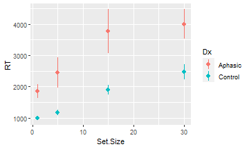<!-- --> --- # A simple MLM example: Fit the models ```r library(lme4) # a null, intercept-only model vs.null <- lmer(RT ~ 1 + (1 + Set.Size | Participant), data=VisualSearchEx, REML=FALSE) # add effect of set size vs <- lmer(RT ~ Set.Size + (Set.Size | Participant), data=VisualSearchEx, REML=F) ``` -- ```r # add effect of diagnosis vs.0 <- lmer(RT ~ Set.Size + Dx + (Set.Size | Participant), data=VisualSearchEx, REML=F) # add set size by diagnosis interaction vs.1 <- lmer(RT ~ Set.Size + Dx + Set.Size:Dx + (Set.Size | Participant), data=VisualSearchEx, REML=F) ``` --- # A simple MLM example: Compare the model fits ```r anova(vs.null, vs, vs.0, vs.1) ``` ``` ## Data: VisualSearchEx ## Models: ## vs.null: RT ~ 1 + (1 + Set.Size | Participant) ## vs: RT ~ Set.Size + (Set.Size | Participant) ## vs.0: RT ~ Set.Size + Dx + (Set.Size | Participant) ## vs.1: RT ~ Set.Size + Dx + Set.Size:Dx + (Set.Size | Participant) ## npar AIC BIC logLik deviance Chisq Df Pr(>Chisq) ## vs.null 5 2283 2297 -1136 2273 ## vs 6 2248 2265 -1118 2236 36.90 1 1.2e-09 *** ## vs.0 7 2241 2261 -1114 2227 8.58 1 0.0034 ** ## vs.1 8 2241 2264 -1113 2225 2.01 1 0.1566 ## --- ## Signif. codes: 0 '***' 0.001 '**' 0.01 '*' 0.05 '.' 0.1 ' ' 1 ``` --- # A simple MLM example: Interpet results <table class="table table-striped table-hover" style="margin-left: auto; margin-right: auto;"> <thead> <tr> <th style="text-align:left;"> </th> <th style="text-align:right;"> npar </th> <th style="text-align:right;"> AIC </th> <th style="text-align:right;"> BIC </th> <th style="text-align:right;"> logLik </th> <th style="text-align:right;"> deviance </th> <th style="text-align:right;"> Chisq </th> <th style="text-align:right;"> Df </th> <th style="text-align:right;"> Pr(&gt;Chisq) </th> </tr> </thead> <tbody> <tr> <td style="text-align:left;"> vs.null </td> <td style="text-align:right;"> 5 </td> <td style="text-align:right;"> 2283 </td> <td style="text-align:right;"> 2297 </td> <td style="text-align:right;"> -1136 </td> <td style="text-align:right;"> 2273 </td> <td style="text-align:right;"> NA </td> <td style="text-align:right;"> NA </td> <td style="text-align:right;"> NA </td> </tr> <tr> <td style="text-align:left;"> vs </td> <td style="text-align:right;"> 6 </td> <td style="text-align:right;"> 2248 </td> <td style="text-align:right;"> 2265 </td> <td style="text-align:right;"> -1118 </td> <td style="text-align:right;"> 2236 </td> <td style="text-align:right;"> 36.902 </td> <td style="text-align:right;"> 1 </td> <td style="text-align:right;"> 0.0000 </td> </tr> <tr> <td style="text-align:left;"> vs.0 </td> <td style="text-align:right;"> 7 </td> <td style="text-align:right;"> 2241 </td> <td style="text-align:right;"> 2261 </td> <td style="text-align:right;"> -1114 </td> <td style="text-align:right;"> 2227 </td> <td style="text-align:right;"> 8.585 </td> <td style="text-align:right;"> 1 </td> <td style="text-align:right;"> 0.0034 </td> </tr> <tr> <td style="text-align:left;"> vs.1 </td> <td style="text-align:right;"> 8 </td> <td style="text-align:right;"> 2241 </td> <td style="text-align:right;"> 2264 </td> <td style="text-align:right;"> -1113 </td> <td style="text-align:right;"> 2225 </td> <td style="text-align:right;"> 2.006 </td> <td style="text-align:right;"> 1 </td> <td style="text-align:right;"> 0.1566 </td> </tr> </tbody> </table> Compared to null model, adding set size (`vs`) substantially improves model fit: response times are affected by number of distractors -- Adding effect of Diagnosis on intercept (`vs.0`) significantly improves model fit: stroke survivors respond more slowly than control participants do -- Adding interaction of set size and Diagnosis, i.e., effect of Diagnosis on slope (`vs.1`), does not significantly improve model fit: stroke survivors are not more affected by distractors than control participants are --- # A simple MLM example: Inspect model .scroll-output[ ```r summary(vs.1) ``` ``` ## Linear mixed model fit by maximum likelihood ['lmerMod'] ## Formula: RT ~ Set.Size + Dx + Set.Size:Dx + (Set.Size | Participant) ## Data: VisualSearchEx ## ## AIC BIC logLik deviance df.resid ## 2241 2264 -1113 2225 124 ## ## Scaled residuals: ## Min 1Q Median 3Q Max ## -3.759 -0.317 -0.079 0.317 6.229 ## ## Random effects: ## Groups Name Variance Std.Dev. Corr ## Participant (Intercept) 613397 783.2 ## Set.Size 380 19.5 1.00 ## Residual 756827 870.0 ## Number of obs: 132, groups: Participant, 33 ## ## Fixed effects: ## Estimate Std. Error t value ## (Intercept) 2078.7 264.4 7.86 ## Set.Size 73.5 11.2 6.54 ## DxControl -1106.1 357.9 -3.09 ## Set.Size:DxControl -21.7 15.2 -1.43 ## ## Correlation of Fixed Effects: ## (Intr) Set.Sz DxCntr ## Set.Size -0.090 ## DxControl -0.739 0.066 ## St.Sz:DxCnt 0.066 -0.739 -0.090 ## optimizer (nloptwrap) convergence code: 0 (OK) ## boundary (singular) fit: see ?isSingular ``` ] --- # A simple MLM example: Parameter p-values Oh no! `summary()` for models fit by `lme4::lmer` (`lmerMod` objects) does not include p-values. ``` ## Estimate Std. Error t value ## (Intercept) 2078.75 264.36 7.863 ## Set.Size 73.49 11.23 6.545 ## DxControl -1106.05 357.95 -3.090 ## Set.Size:DxControl -21.74 15.20 -1.430 ``` Those p-values are one-sample t-tests of whether `\(Est \neq 0\)` with `\(t = Est/SE\)` -- The `df` for these t-tests are not simple to determine because random effects are not free parameters (estimated under constraints). But `df` can be estimated, and the two most common estimations are "Kenward-Roger" and "Satterthwaite". These approximations are implemented in a few different packages (`afex`, `lmerTest`, `pbkrtest`). --- # A simple MLM example: Parameter p-values One of the easiest to use is the `lmerTest` package: you can fit the model the same way (it just passes your call to `lmer`) and it will calculate the Satterthwaite approximation and add those `df` and p-values to the model summary -- .scroll-output[ ```r library(lmerTest) vs.1 <- lmer(RT ~ Set.Size + Dx + Set.Size:Dx + (Set.Size | Participant), data=VisualSearchEx, REML=F) summary(vs.1) ``` ``` ## Linear mixed model fit by maximum likelihood . t-tests use Satterthwaite's ## method [lmerModLmerTest] ## Formula: RT ~ Set.Size + Dx + Set.Size:Dx + (Set.Size | Participant) ## Data: VisualSearchEx ## ## AIC BIC logLik deviance df.resid ## 2241 2264 -1113 2225 124 ## ## Scaled residuals: ## Min 1Q Median 3Q Max ## -3.759 -0.317 -0.079 0.317 6.229 ## ## Random effects: ## Groups Name Variance Std.Dev. Corr ## Participant (Intercept) 613397 783.2 ## Set.Size 380 19.5 1.00 ## Residual 756827 870.0 ## Number of obs: 132, groups: Participant, 33 ## ## Fixed effects: ## Estimate Std. Error df t value Pr(>|t|) ## (Intercept) 2078.7 264.4 35.7 7.86 2.6e-09 *** ## Set.Size 73.5 11.2 54.9 6.54 2.1e-08 *** ## DxControl -1106.1 357.9 35.7 -3.09 0.0039 ** ## Set.Size:DxControl -21.7 15.2 54.9 -1.43 0.1585 ## --- ## Signif. codes: 0 '***' 0.001 '**' 0.01 '*' 0.05 '.' 0.1 ' ' 1 ## ## Correlation of Fixed Effects: ## (Intr) Set.Sz DxCntr ## Set.Size -0.090 ## DxControl -0.739 0.066 ## St.Sz:DxCnt 0.066 -0.739 -0.090 ## optimizer (nloptwrap) convergence code: 0 (OK) ## boundary (singular) fit: see ?isSingular ``` ] --- # A simple MLM example: Plot model fit ```r ggplot(VisualSearchEx, aes(Set.Size, RT, color=Dx)) + stat_summary(fun.data=mean_se, geom="pointrange") + stat_summary(aes(y=fitted(vs.0)), fun=mean, geom="line") ``` 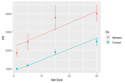<!-- --> --- # Another way to plot model fit The `effects` package provides a convenient way to pull estimated values from a model (along with SE and confidence intervals). Very useful for plotting effects from complicated models, or when there are missing data, etc. ```r library(effects) ef <- as.data.frame(effect("Set.Size:Dx", vs.0)) head(ef) ``` ``` ## Set.Size Dx fit se lower upper ## 1 1.0 Aphasic 2162 262.3 1643.0 2681 ## 2 8.2 Aphasic 2606 266.8 2077.8 3133 ## 3 16.0 Aphasic 3086 284.1 2524.3 3649 ## 4 23.0 Aphasic 3518 309.0 2906.5 4129 ## 5 30.0 Aphasic 3949 340.7 3275.3 4623 ## 6 1.0 Control 1016 239.4 542.7 1490 ``` --- # Another way to plot model fit The `effects` package provides a convenient way to pull estimated values from a model (along with SE and confidence intervals). Very useful for plotting effects from complicated models, or when there are missing data, etc. ```r ggplot(ef, aes(Set.Size, fit, color=Dx)) + geom_line() ``` <!-- --> --- # Some general advice This semester you will be learning statistical methods that don't have "cookbook" recipes. You'll need to actively engage with the data and research question in order to come up with a good model for answering the question, then to defend/explain that model. -- **Practice is absolutely critical** to learning how to do this. You can't learn it just from the lectures; you have to try it with real data. You will make mistakes, run into problems, etc. Identifying the mistakes and solving those problems is how you'll master this material. *We have made all of the example data sets and code available to you for exactly this reason.* -- Do the lab exercises! If you're not sure, **try something** then try to figure out whether it worked or not. Ask questions when you're stuck -- we're here to help you learn, but it will only work if you engage in **active, hands-on learning**.  --- # Live R Questions? -- ### Use MLM to run a 2x2 repeated-measures ANOVA -- Recall: 1. ANOVA is a particular kind of GLM (linear regression with categorical predictors). 2. Repeated-measures ANOVA is used for within-participant manipulations; aka, nested observations. -- MLM is an extension of GLM with random effects to capture within-participant nesting, so we should be able to implement a 2x2 rm-ANOVA using MLM. -- **Example 1**: Fazio (2020) Repetition Increases Perceived Truth Even for Known Falsehoods. *Collabra: Psychology, 6*(1):38. https://doi.org/10.1525/collabra.347. Data available at: https://osf.io/kt2p8/ Participants had to determine whether statements were true or false. The manipulations were (1) whether the fact was known or unknown to the participant and (2) whether the participant had been previously exposed to the statement. We know repeated exposure increases "truthiness" of false statements, the key question is whether prior knowledge is a protective factor. That is, does *knowing* that the statement is false protect people from the repetition effect?